Add Transparency to Plots
WORKFLOW
Add Transparency to Plots
Create unobstructed views of multiple components of one plot or lighten a single plot component against the background.
Using 2D Plots...
Create a plot
Use Plot to create a graph of ![]() :
:
eq = x ^ 2Plot[eq, {x, -2, 2}]Add options to the plot
Use the PlotStyle option with Opacity to make the plot 70% transparent:
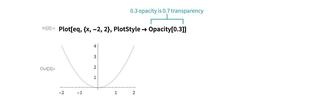
- Opacity is an OptionValue for PlotStyle.
Add different transparency settings for plots of multiple functions:
eq2 = -x ^ 2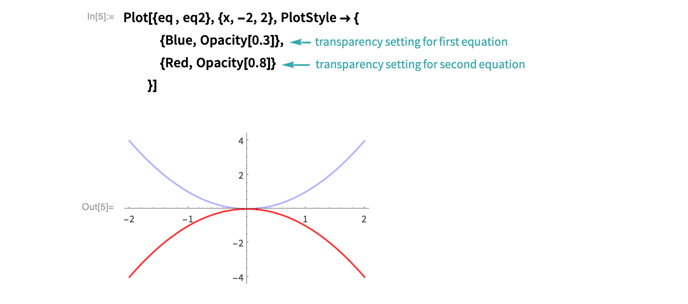
Using 3D Plots...
Create a plot
Use Plot3D to create a graph of the polynomial ![]() :
:
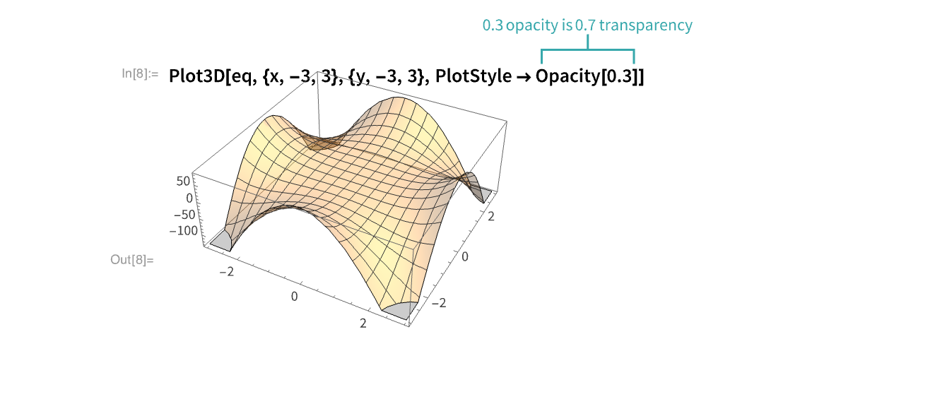
eq = x ^ 4 + y ^ 4 - 5 x ^ 2 * y ^ 2Plot3D[eq, {x, -3, 3}, {y, -3, 3}]Add options to the plot
Use the PlotStyle option with Opacity to make the plot 70% transparent:
Add different transparency settings for plots of multiple functions:
eq2 = -100 - x ^ 4 - y ^ 4 + 5 x ^ 2 * y ^ 2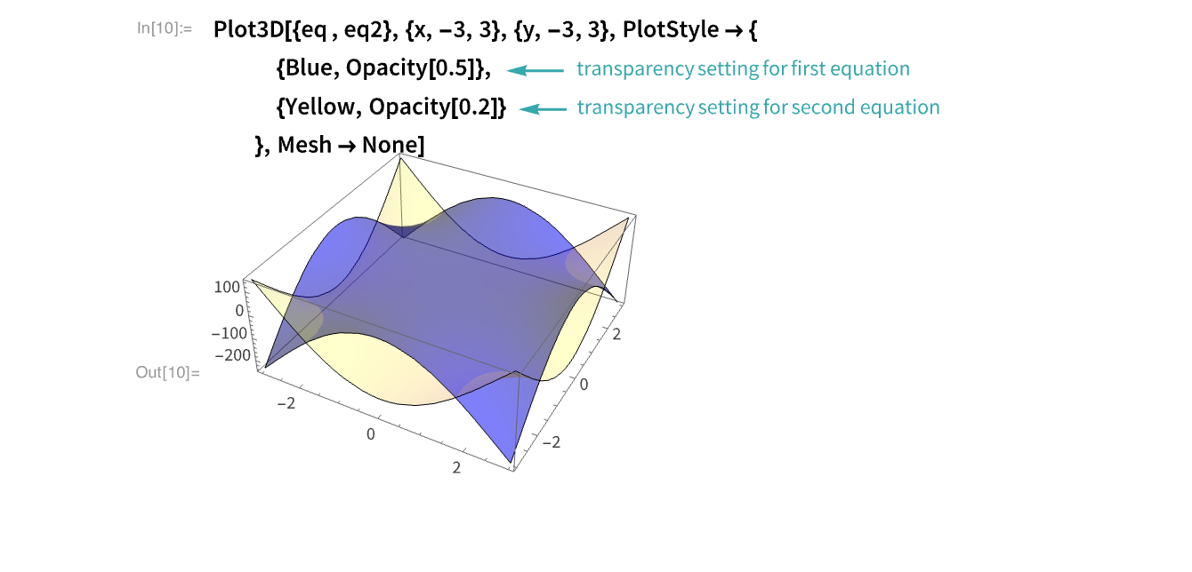
Using Graphics...
Create a disk graphic
Apply Graphics to Disk to render a unit disk:
Graphics[Disk[]]Add options to the graphic
Make a 75% transparent disk:
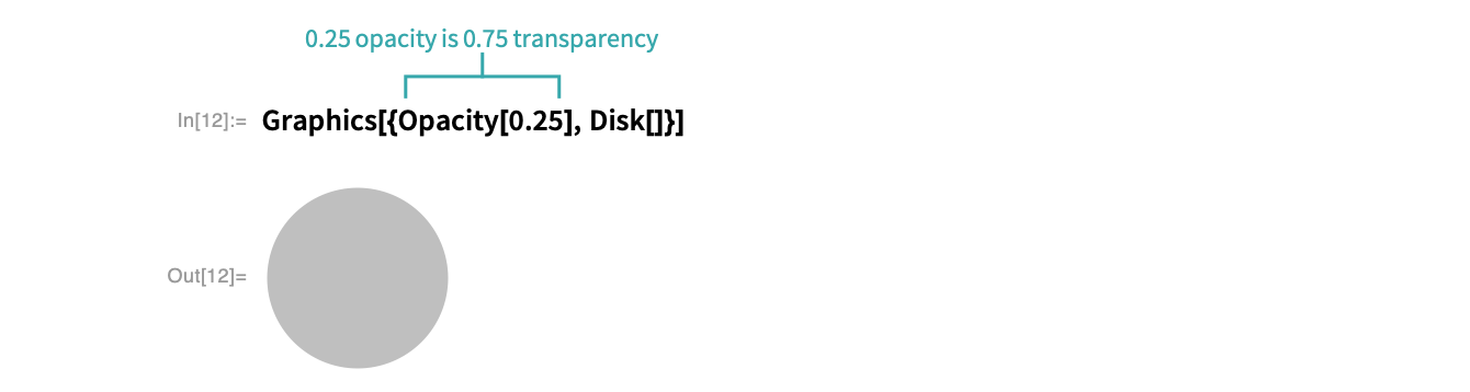
Opacity can have values between 0 and 1, with 0 corresponding to perfect transparency:
Row[Table[
	Graphics[{Opacity[n], Disk[]}, ImageSize -> Scaled[.1]],
	{n, 0.1, 1, 0.3}]]
Use Opacity with a color:
Row[Table[
	Graphics[{Red, Opacity[n], Disk[]}, ImageSize -> Scaled[.1]],
	{n, 0.1, 1, 0.3}]]
Notes
Opacity interacts well with other functions:
Manipulate[RegionPlot[
	{x - y ≥ t, x + y ≥ s}, {x, -3 Pi, 3 Pi}, {y, -3 Pi, 3 Pi},
	PlotPoints -> 30,
	PlotStyle -> {Directive[Red], Directive[Blue, Opacity[0.5]]}
	],
	Style["Solving the system of inequalities: x-y ≥ t and x +y ≥ s", Bold, 12],
	{{s, 0}, -20, 20}, {{t, 0}, -20, 20}
	]