

CompleteIntegral
CompleteIntegral[pde,u,{x1,…,xn}]
gives a complete integral u for the first-order partial differential equation pde, with independent variables {x1,…,xn}.
Details and Options
- A complete integral of a first-order partial differential equation (PDE) in n variables is a solution that depends on n independent arbitrary constants c1,c2,…,cn.
- A complete integral is typically used to generate a complete set of solutions to the PDE.
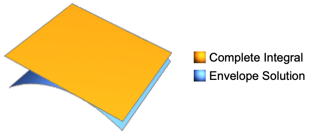
- A solution to the PDE that satisfies a specific initial condition can be obtained by constructing the envelope of a smoothly varying subfamily of simple solutions that depend on
 parameters, as illustrated. »
 - The output from CompleteIntegral is controlled by the form of the dependent function u or u[x1,…,xn], as in DSolve.
- CompleteIntegral can give implicit solutions in terms of Solve.
- CompleteIntegral can give solutions that include Inactive sums and integrals that cannot be carried out explicitly. Variables K[1], K[2], … are used in such cases.
- Boundary conditions for the PDE can be specified to obtain specific solutions of the PDE that are free from the arbitrary constants in the complete integral. »
- The following options can be given:
-
Assumptions $Assumptions assumptions on parameters GeneratedParameters C how to name generated parameters Method Automatic what method to use - GeneratedParameters controls the form of generated parameters; these are by default constants C[n].
Examples
open all close allBasic Examples (3)
Find a complete integral of a partial differential equation:
CompleteIntegral[D[u[x, y], x] - D[u[x, y], y] ^ 2 == Cos[x] , u[x, y], {x, y}]Plot the solution for particular values of the arbitrary constants:
Plot3D[u[x, y] /. %[[1]] /. {C[1] -> 1 / 3, C[2] -> 1}, {x, 0, 10Pi}, {y, 0, 5}]Get a "pure function" complete integral for w:
CompleteIntegral[D[w[x, y], x] - y w[x, y]D[w[x, y], y] == w[x, y] + x ^ 2 - 1, w, {x, y}]Substitute the solution into an expression:
Simplify[D[w[x, y], x] - y w[x, y]D[w[x, y], y] == w[x, y] + x ^ 2 - 1 /. %]Complete integral of a partial differential equation in 3 dimensions:
CompleteIntegral[D[u[x, y, z], x] ^ 3 == D[u[x, y, z], y] + D[u[x, y, z], z], u[x, y, z], {x, y, z}]CompleteIntegral[D[u[x, y, z], x] ^ 3 == D[u[x, y, z], y] + D[u[x, y, z], z] && u[0, 1, 1] == 1 && u[1, 0, 1] == 1 && u[0, 0, 1] == 1 / 2, u[x, y, z], {x, y, z}]Scope (5)
Find the complete integral of a partial differential equation in 2 dimensions:
CompleteIntegral[D[u[x, y], x] + D[u[x, y], y] == u[x, y] ^ 2, u[x, y], {x, y}]Get a "pure function" complete integral for u:
CompleteIntegral[D[u[x, y], x] + D[u[x, y], y] == u[x, y] ^ 2, u, {x, y}]Substitute the solution into an expression:
Simplify[D[u[x, y], x] + D[u[x, y], y] /. %]Complete integral that can be expressed using elementary functions:
CompleteIntegral[D[w[x, y], x] - 1 / Sin[y]w[x, y]D[w[x, y], y] == 1 / x w[x, y] + Log[x], w[x, y], {x, y}]Complete integral that can be expressed using special functions:
CompleteIntegral[D[w[x, y], x] - y w[x, y]D[w[x, y], y] == x w[x, y] + x ^ 2 - 1, w[x, y], {x, y}]Complete integral for a linear PDE:
CompleteIntegral[ D[u[x, y], x] - x D[u[x, y], y] == 0, u[x, y], {x, y}]Compare with the solution given by DSolve:
DSolve[ D[u[x, y], x] - x D[u[x, y], y] == 0, u[x, y], {x, y}]Complete integral for a quasi-linear PDE:
CompleteIntegral[ D[u[x, y], x] - u[x, y] D[u[x, y], y] == 0, u[x, y], {x, y}]Compare with the solution given by DSolve:
DSolve[ D[u[x, y], x] - u[x, y] D[u[x, y], y] == 0, u[x, y], {x, y}]Applications (2)
Find a complete integral of the Clairaut equation:
ClairautEquation = u[x, y] == x * D[u[x, y], {x}] + y * D[u[x, y], {y}] +
     (1 / 2) * (D[u[x, y], {x}] ^ 2 + D[u[x, y], {y}] ^ 2);
The complete integral is given by a two-parameter family of planes:
csol = u[x, y] /. CompleteIntegral[ClairautEquation, u, {x, y}][[1]]Select a one-parameter family of these planes:
psol = csol /. {C[2] -> -1}Find the envelope of this one-parameter family of planes:
Solve[(D[psol, C[1]]) == 0, C[1]]envelope = psol /. %[[1]]//TogetherVerify that the envelope is also a solution:
ClairautEquation /. {u -> Function[{x, y}, Evaluate[envelope]]}//SimplifyVisualize the one-parameter family of planes and the envelope solution:
Animate[...]Find a complete integral of the Hamilton–Jacobi equation:
HamiltonJacobiEqn = D[u[t, x], t] + D[u[t, x], x] ^ 2 == 0;ci = CompleteIntegral[HamiltonJacobiEqn, u[t, x], {t, x}]Compute an envelope solution for the equation:
sol = u[t, x] /. ci[[1]] /. {C[1] -> 0, C[2] -> a}Solve[D[sol, a] == 0, a]envelopsol = sol /. %[[1]]Plot3D[Evaluate[envelopsol], {t, -4, 4}, {x, -3, 3}, PlotRange -> All]Verify that the envelope solution satisfies the equation:
HamiltonJacobiEqn /. u -> Function[{t, x}, Evaluate[envelopsol]]Properties & Relations (2)
CompleteIntegral finds a complete integral for a nonlinear PDE:
deqn = D[u[x, y], x] + D[u[x, y], y] ^ 2 == 1;CompleteIntegral[deqn, u[x, y], {x, y}]DSolve returns the same solution with a warning message:
DSolve[deqn, u[x, y], {x, y}]Use CompleteIntegral to find a complete integral for a linear PDE:
deqn = D[u[x, y], x] + D[u[x, y], y] == 1;CompleteIntegral[deqn, u[x, y], {x, y}]DSolve returns the general solution for this PDE:
DSolve[deqn, u[x, y], {x, y}]Text
Wolfram Research (2021), CompleteIntegral, Wolfram Language function, https://reference.wolfram.com/language/ref/CompleteIntegral.html.
CMS
Wolfram Language. 2021. "CompleteIntegral." Wolfram Language & System Documentation Center. Wolfram Research. https://reference.wolfram.com/language/ref/CompleteIntegral.html.
APA
Wolfram Language. (2021). CompleteIntegral. Wolfram Language & System Documentation Center. Retrieved from https://reference.wolfram.com/language/ref/CompleteIntegral.html