


ConnectSystemModelController
ConnectSystemModelController[model,controller]
connects the system model model with a controller according to the controller data controller.
Details
- ConnectSystemModelController is typically used to connect a controller to a SystemModel plant model and give the closed-loop system back. The resulting system can then be simulated and analyzed for real-world performance.
- The model can be a SystemModel object, a full model name string or a shortened model name accepted by SystemModel.
- ConnectSystemModelController["NewModel",…] gives the created model the name "NewModel".
- The controller is a SystemsModelControllerData object produced by control design functions.
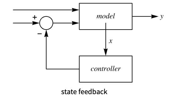
- With state feedback from model, the control design functions include:
-
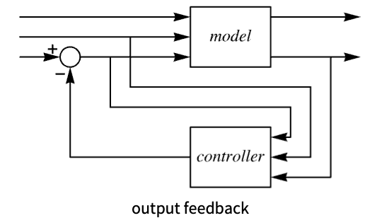
StateFeedbackGains pole placement state feedback LQRegulatorGains linear quadratic optimal control DiscreteLQRegulatorGains discrete-time linear quadratic optimal control ModelPredictiveController constrained model predictive controller - With output feedback from model, the controller design functions include:
-
EstimatorRegulator assembling state feedback and state estimator LQGRegulator linear quadratic control and estimator PIDTune automatically tuned PID controller - ConnectSystemModelController returns a SystemModel.
Examples
open all close allBasic Examples (1)
Start with a model for a DC motor:
model = [image];Linearize it around an equilibrium point and create a controller:
ctrl = PIDTune[SystemModelLinearize[model], Automatic, "Data"]Generate the closed-loop system for the controlled model:
csys = ConnectSystemModelController[model, ctrl]Provide a reference input and plot the output:
SystemModelPlot[csys, {"out"}, 10, <|"Inputs" -> {"ref" -> Function[2], "ctrlDist" -> Cos, "sensNoise" -> Sin}|>, PlotRange -> All]Scope (16)
StateFeedbackGains (3)
Start with a model for a submerging submarine:
model = [image];Linearize it around an equilibrium point:
lin = SystemModelLinearize[model]ctrl = StateFeedbackGains[<|"InputModel" -> lin, "FeedbackInputs" -> {1}|>, {-2 + I, -2 - I}, "Data"]Generate the closed-loop system for the controlled model:
csys = ConnectSystemModelController[model, ctrl]Perturb the submarine with a vertical force:
simModel = SystemModelSimulate[model, 10, <|"Inputs" -> {"f" -> Function[t, 10^8(UnitStep[t] - UnitStep[t - 1])], "deltarho" -> Function[0]}|>]Simulate the closed-loop system with the same disturbance:
simCsys = SystemModelSimulate[csys, 10, <|"Inputs" -> {"f" -> Function[t, 10^8(UnitStep[t] - UnitStep[t - 1])], "deltarho" -> Function[0]}|>]Plot the depth of the submarine in the original model:
SystemModelPlot[simModel, {"y"}]In the closed-loop system, the submarine changes its density to preserve its depth:
SystemModelPlot[simCsys, {"y"}]Start with a model for a spacecraft in a circular orbit:
model = [image];Linearize it around an equilibrium point:
lin = SystemModelLinearize[model]ctrl = StateFeedbackGains[lin, {-0.5, -1.5, -1, -2.5}, "Data"]Generate the closed-loop system for the controlled model:
csys = ConnectSystemModelController[model, ctrl]Simulate the original model with an initial velocity:
simModel = SystemModelSimulate[model, 20, <|"InitialValues" -> {"keplerDynamics.vx" -> 0.1}|>]Simulate the closed-loop system with the same initial velocity:
simCsys = SystemModelSimulate[csys, 20, <|"InitialValues" -> {"eSys.sys.keplerDynamics.vx" -> 0.1}|>]Plot the deviations from the circular trajectory in the original model:
Row[Table[SystemModelPlot[simModel, {var}, TargetUnits -> {"Seconds", Automatic}, PlotRange -> All, PlotLabel -> var, ImageSize -> 225], {var, {"dphi", "dr"}}]]The closed-loop system brings the spacecraft back to its circular orbit:
Row[Table[SystemModelPlot[simCsys, {var}, TargetUnits -> {"Seconds", Automatic}, PlotRange -> All, PlotLabel -> var, ImageSize -> 225], {var, {"dphi", "dr"}}]]Start with a model for an inverted pendulum:
model = \!\(\*GraphicsBox[«8»]\);Linearize it around an equilibrium point:
lin = SystemModelLinearize[model]ctrl = StateFeedbackGains[<|"InputModel" -> lin, "FeedbackInputs" -> {2}|>, {-9 + 9I, -9 - 9I, -10, -10.5}, "Data"]Generate the closed-loop system for the controlled model:
csys = ConnectSystemModelController[model, ctrl]Apply a tangential force to the pendulum and simulate it:
simModel = SystemModelSimulate[model, 5, <|"Inputs" -> {"d" -> Function[t, 0.1(UnitStep[t] - UnitStep[t - 1])], "f" -> Function[0]}|>]Simulate the closed-loop system with the same disturbance:
simCsys = SystemModelSimulate[csys, 5, <|"Inputs" -> {"d" -> Function[t, 0.1(UnitStep[t] - UnitStep[t - 1])], "f" -> Function[0]}|>]Plot the angle of the pendulum in the original model:
SystemModelPlot[simModel, {"phi"}, PlotRange -> All]The closed-loop system applies a horizontal force and brings the pendulum back to the vertical position:
SystemModelPlot[simCsys, {"phi"}, PlotRange -> All]LQRegulatorGains (2)
Start with a model for a continuous stirred-tank reactor:
model = [image];Linearize it around an equilibrium point:
lin = SystemModelLinearize[model]ctrl = LQRegulatorGains[lin, {(| | | |
| - | - | - |
| 1 | 0 | 0 |
| 0 | 1 | 0 |
| 0 | 0 | 1 |), {{1}}}, "Data"]Generate the closed-loop system:
csys = ConnectSystemModelController[model, ctrl]Simulate the original model with a deficit in the concentration of the reactant from its equilibrium value:
simModel = SystemModelSimulate[model, Quantity[1, "Hours"], <|"InitialValues" -> {"x1" -> -1000}|>]Simulate the closed-loop system with the same initial condition:
simCsys = SystemModelSimulate[csys, Quantity[1, "Hours"], <|"InitialValues" -> {"eSys.sys.x1" -> -1000}|>]Plot the change in reactant concentration in the original model:
SystemModelPlot[simModel, {"deltaCA"}, PlotRange -> All, TargetUnits -> {"Hours", None}]The closed-loop system controls the flow rate and brings the concentration back to the equilibrium value:
SystemModelPlot[simCsys, {"deltaCA"}, PlotRange -> All, TargetUnits -> {"Hours", None}]Start with a model for a ball placed on top of a beam that can rotate around its center of mass:
model = SystemModel[[image], <|"ParameterValues" -> {"world.enableAnimation" -> False}|>];Linearize it around an equilibrium point:
lin = SystemModelLinearize[model]ctrl = LQRegulatorGains[lin, {(| | | | |
| - | - | - | - |
| 1 | 0 | 0 | 0 |
| 0 | 1 | 0 | 0 |
| 0 | 0 | 1 | 0 |
| 0 | 0 | 0 | 1 |), (1)}, "Data"]Generate the closed-loop system:
csys = ConnectSystemModelController[model, ctrl]Simulate the original model placing the ball at the edge of the beam:
simModel = SystemModelSimulate[model, 10, <|"InitialValues" -> {"ballAndBeamDynamics.rs" -> 0.4}|>]Simulate the closed-loop system with the same initial condition:
simCsys = SystemModelSimulate[csys, 10, <|"InitialValues" -> {"eSys.sys.ballAndBeamDynamics.rs" -> 0.4}|>]Plot the position of the ball, measured from the middle of the beam, in the original model:
SystemModelPlot[simModel, {"ballAndBeamDynamics.rs"}]The closed-loop system applies a torque and brings the ball back to the middle of the beam:
SystemModelPlot[simCsys, {"eSys.sys.ballAndBeamDynamics.rs"}, PlotRange -> All]DiscreteLQRegulatorGains (2)
Start with a model for a continuous stirred-tank reactor:
model = [image];Linearize it around an equilibrium point:
lin = SystemModelLinearize[model]ctrl = DiscreteLQRegulatorGains[lin, {(| | | |
| - | - | - |
| 1 | 0 | 0 |
| 0 | 1 | 0 |
| 0 | 0 | 1 |), {{1}}}, 60, "Data"]Generate the closed-loop system:
csys = ConnectSystemModelController[model, ctrl]Simulate the original model with a deficit in the concentration of the reactant from its equilibrium value:
simModel = SystemModelSimulate[model, Quantity[4, "Hours"], <|"InitialValues" -> {"x1" -> -1000}|>]Simulate the closed-loop system with the same initial condition:
simCsys = SystemModelSimulate[csys, Quantity[4, "Hours"], <|"InitialValues" -> {"eSys.sys.x1" -> -1000}|>]Plot the change in reactant concentration in the original model:
SystemModelPlot[simModel, {"deltaCA"}, PlotRange -> All, TargetUnits -> {"Hours", None}]The closed-loop system controls the flow rate and brings the concentration back to the equilibrium value:
SystemModelPlot[simCsys, {"deltaCA"}, PlotRange -> All, TargetUnits -> {"Hours", None}]Start with a model for a ball placed on top of a beam that can rotate around its center of mass:
model = SystemModel[[image], <|"ParameterValues" -> {"world.enableAnimation" -> False}|>];Linearize it around an equilibrium point:
lin = SystemModelLinearize[model]ctrl = DiscreteLQRegulatorGains[lin, {(| | | | |
| - | - | - | - |
| 1 | 0 | 0 | 0 |
| 0 | 1 | 0 | 0 |
| 0 | 0 | 1 | 0 |
| 0 | 0 | 0 | 1 |), (1)}, 0.1, "Data"]Generate the closed-loop system:
csys = ConnectSystemModelController[model, ctrl]Simulate the original model placing the ball at the edge of the beam:
simModel = SystemModelSimulate[model, 10, <|"InitialValues" -> {"ballAndBeamDynamics.rs" -> 0.4}|>]Simulate the closed-loop system with the same initial condition:
simCsys = SystemModelSimulate[csys, 10, <|"InitialValues" -> {"eSys.sys.ballAndBeamDynamics.rs" -> 0.4}|>]Plot the position of the ball, measured from the middle of the beam, in the original model:
SystemModelPlot[simModel, {"ballAndBeamDynamics.rs"}]The closed-loop system applies a torque and brings the ball back to the middle of the beam:
SystemModelPlot[simCsys, {"eSys.sys.ballAndBeamDynamics.rs"}, PlotRange -> All]EstimatorRegulator (2)
Start with a model for a spacecraft in a circular orbit:
model = [image];Linearize it around an equilibrium point:
lin = SystemModelLinearize[model]Design a controller and observer and put them together in EstimatorRegulator:
k = StateFeedbackGains[lin, {-0.5, -1.5, -1, -2.5}];l = EstimatorGains[lin, 3 {-0.5, -1.5, -1, -2.5}];ctrl = EstimatorRegulator[lin, {l, k}, "Data"]Generate the closed-loop system for the controlled model:
csys = ConnectSystemModelController[model, ctrl]Simulate the closed-loop system with an initial velocity:
simCSys = SystemModelSimulate[csys, 12, <|"InitialValues" -> {"sys.keplerDynamics.vx" -> 0.1}|>]The closed-loop system brings the spacecraft back to its circular orbit:
SystemModelPlot[simCSys, {"dr"}, PlotRange -> All]Start with a model for an inverted pendulum:
model = \!\(\*GraphicsBox[«8»]\);Linearize it around an equilibrium point:
lin = SystemModelLinearize[model]Design a controller and observer and put them together in EstimatorRegulator:
sysSpec = <|"InputModel" -> lin, "FeedbackInputs" -> {2}|>;k = StateFeedbackGains[sysSpec, {-1 + 1.5I, -1 - 1.5I, -5, -5.5}];l = EstimatorGains[lin, {-9 + 9I, -9 - 9I, -10, -10.5}];ctrl = EstimatorRegulator[sysSpec, {l, k}, "Data"]Generate the closed-loop system for the controlled model:
csys = ConnectSystemModelController[model, ctrl]Simulate the closed-loop system with an initial angle away from the equilibrium:
simCsys = SystemModelSimulate[csys, 10, <|"InitialValues" -> {"sys.pendulumDamper.phi_rel" -> 0.1}|>]The closed-loop system applies forces to bring the pendulum back to vertical position:
SystemModelPlot[simCsys, {"sys.pendulumDamper.phi_rel"}, PlotRange -> All]LQGRegulator (2)
Start with a model for a continuous stirred-tank reactor:
model = [image];Linearize it around an equilibrium point:
lin = SystemModelLinearize[model]ctrl = LQGRegulator[lin, {{{}}, (| | | |
| - | - | - |
| 1 | 0 | 0 |
| 0 | 1 | 0 |
| 0 | 0 | 1 |)}, {(| | | |
| - | - | - |
| 1 | 0 | 0 |
| 0 | 1 | 0 |
| 0 | 0 | 1 |), (1)}, "Data"]Generate the closed-loop system for the controlled model:
csys = ConnectSystemModelController[model, ctrl]Simulate the original model with a deficit in the concentration of the reactant from its equilibrium value:
simCsys = SystemModelSimulate[csys, Quantity[8, "Hours"], <|"InitialValues" -> {"sys.x1" -> -1000}|>]The closed-loop system controls the flow rate and brings the concentration back to the equilibrium value:
SystemModelPlot[simCsys, {"deltaCA"}, PlotRange -> All, TargetUnits -> {"Hours", None}]Start with a model for a ball placed on top of a beam that can rotate around its center of mass and add some rotational damping:
model = SystemModel[[image], <|"ParameterValues" -> {"b" -> 1, "world.enableAnimation" -> False}|>];Linearize it around an equilibrium point:
lin = SystemModelLinearize[model]ctrl = LQGRegulator[lin, {{{}}, (| | |
| ----- | ----- |
| 10^-6 | 0 |
| 0 | 10^-6 |)}, {(| | | | |
| ---- | ---- | ---- | ---- |
| 10^4 | 0 | 0 | 0 |
| 0 | 10^4 | 0 | 0 |
| 0 | 0 | 10^4 | 0 |
| 0 | 0 | 0 | 10^4 |), (1)}, "Data"]Generate the closed-loop system for the controlled model:
csys = ConnectSystemModelController[model, ctrl]Simulate the closed-loop system placing the ball away from the middle of the beam:
simCsys = SystemModelSimulate[csys, 20, <|"InitialValues" -> {"sys.ballAndBeamDynamics.rs" -> 0.4}|>]The closed-loop system applies a torque and brings the ball back to the middle of the beam:
SystemModelPlot[simCsys, {"sys.ballAndBeamDynamics.rs"}, PlotRange -> All]PIDTune (1)
Start with a model for an RLC circuit:
model = [image];Linearize it around an equilibrium point:
lin = SystemModelLinearize[model]ctrl = PIDTune[lin, Automatic, "Data"]Generate the closed-loop system for the controlled model:
csys = ConnectSystemModelController[model, ctrl]Provide a reference input and plot the output:
SystemModelPlot[csys, {"out"}, 0.1, <|"Inputs" -> {"ref" -> Function[2], "ctrlDist" -> Cos, "sensNoise" -> Sin}|>, PlotRange -> All]ModelPredictiveController (2)
Start with a model for a camera stabilizer:
model = \!\(\*GraphicsBox[«8»]\);Linearize it around an equilibrium point:
SystemModelLinearize[model]sspec = <|"InputModel" -> model, "SamplingPeriod" -> 0.05, "SamplingMethod" -> "ForwardRectangularRule", "FeedbackInputs" -> {"fa"}|>;cost = <|"Horizon" -> 3, "StateWeight" -> (| | | | | | |
| - | ---- | - | - | ---- | - |
| 1 | 0 | 0 | 0 | 0 | 0 |
| 0 | 10^6 | 0 | 0 | 0 | 0 |
| 0 | 0 | 1 | 0 | 0 | 0 |
| 0 | 0 | 0 | 1 | 0 | 0 |
| 0 | 0 | 0 | 0 | 10^6 | 0 |
| 0 | 0 | 0 | 0 | 0 | 1 |), "InputWeight" -> (1)|>;cons = {-0.1 <= "xce" <= 0.1};ctrl = ModelPredictiveController[sspec, cost, cons]Generate the closed-loop system for the controlled model:
csys = ConnectSystemModelController["CLSMPC", model, ctrl]Perturb the system with a vertical force:
bumpInputs = <|"Inputs" -> {"fa" -> Function[t, 0], "fw" -> Function[t, 2000(UnitStep[t] - UnitStep[t - 0.25])]}|>;simModel = SystemModelSimulate[model, 10, bumpInputs]Simulate the closed-loop system with the same disturbance:
simCsys = SystemModelSimulate[csys, 10, bumpInputs]Plot the position of the camera in the original model:
SystemModelPlot[simModel, {"xce"}, PlotRange -> {-0.025, 0.025}]In the closed-loop system, the position of the camera does not change as much:
SystemModelPlot[simCsys, {"eSys.sys.xce"}, PlotRange -> {-0.025, 0.025}]Start with a model for a continuous stirred-tank reactor:
model = [image];Linearize it around an equilibrium point:
SystemModelLinearize[model]sspec = <|"InputModel" -> model, "SamplingPeriod" -> 60, "SamplingMethod" -> "ForwardRectangularRule"|>;cost = <|"Horizon" -> ∞, "StateWeight" -> (| | | |
| - | - | - |
| 1 | 0 | 0 |
| 0 | 1 | 0 |
| 0 | 0 | 1 |), "InputWeight" -> (1)|>;cons = {-50 ≤ "deltaCA" ≤ 50};ctrl = ModelPredictiveController[sspec, cost, cons]Generate the closed-loop system for the controlled model:
csys = ConnectSystemModelController["CLSMPC", model, ctrl]Simulate the original model with a deficit in the concentration of the reactant from its equilibrium value:
simModel = SystemModelSimulate[model, Quantity[4, "Hours"], <|"InitialValues" -> {"x1" -> -20}|>]Simulate the closed-loop system with the same initial condition:
simCsys = SystemModelSimulate[csys, Quantity[4, "Hours"], <|"InitialValues" -> {"eSys.sys.x1" -> -20}|>]Plot the change in reactant concentration in the original model:
SystemModelPlot[simModel, {"x1"}, PlotRange -> All, TargetUnits -> {"Hours", Automatic}]The closed-loop system controls the flow rate and brings the concentration back to the equilibrium value:
SystemModelPlot[simCsys, {"eSys.sys.x1"}, PlotRange -> All, TargetUnits -> {"Hours", Automatic}]Tracking (2)
Start with a model for a submarine:
model = [image];Linearize it around an equilibrium point:
lin = SystemModelLinearize[model]Design a controller that tracks the depth of the submarine:
sspec = <|"InputModel" -> lin, "FeedbackInputs" -> {1}, "TrackedOutputs" -> {1}|>;ctrl = StateFeedbackGains[sspec, {-2 + I, -2 - I, -2}, "Data"]Generate the closed-loop system for the controlled model:
csys = ConnectSystemModelController[model, ctrl]Simulate the closed-loop system providing a reference signal for the depth and noise:
sim = SystemModelSimulate[csys, 100, <|"Inputs" -> {"refY" -> Function[t, -10Tanh[t / 10]], "f" -> RandomFunction[WienerProcess[0, 10^6], {0, 100, 0.1}]}|>]Plot the reference and the output:
SystemModelPlot[sim, {"refY", "y"}, PlotRange -> All]Plot the density change needed to reproduce the reference:
SystemModelPlot[sim, {"eSys.sys.deltarho"}, PlotRange -> All]Start with a model for a ball placed on top of a beam that can rotate around its center of mass:
model = SystemModel[[image], <|"ParameterValues" -> {"world.enableAnimation" -> False}|>];Linearize it around an equilibrium point:
lin = SystemModelLinearize[model]Design a controller that tracks the position of the ball:
sspec = <|"InputModel" -> lin, "TrackedOutputs" -> {1}|>;ctrl = LQGRegulator[sspec, {{{}}, (| | |
| ----- | ----- |
| 10^-5 | 0 |
| 0 | 10^-5 |)}, {10^4(| | | | | |
| - | - | - | - | - |
| 1 | 0 | 0 | 0 | 0 |
| 0 | 1 | 0 | 0 | 0 |
| 0 | 0 | 1 | 0 | 0 |
| 0 | 0 | 0 | 1 | 0 |
| 0 | 0 | 0 | 0 | 1 |), (1)}, "Data"]Generate the closed-loop system for the controlled model:
csys = ConnectSystemModelController[model, ctrl]Simulate the closed-loop system providing a reference signal for the position and noise:
sim = Quiet[SystemModelSimulate[csys, 100, <|"Inputs" -> {"refRs" -> Function[t, 1 / 2 E ^ (-(1 / 8) (-10 + t) ^ 2)], "noiseRs" -> RandomFunction[WienerProcess[0, 0.0001], {0, 100, 0.01}], "noiseThetab" -> RandomFunction[WienerProcess[0, 0.00001], {0, 100, 0.01}]}|>], {General::munfl}]Plot the reference and the output:
SystemModelPlot[sim, {"rs", "refRs"}, PlotRange -> All]Plot the input torque needed to reproduce the reference:
SystemModelPlot[sim, {"sys.T"}, PlotRange -> All]Related Links
Text
Wolfram Research (2021), ConnectSystemModelController, Wolfram Language function, https://reference.wolfram.com/language/ref/ConnectSystemModelController.html (updated 2022).
CMS
Wolfram Language. 2021. "ConnectSystemModelController." Wolfram Language & System Documentation Center. Wolfram Research. Last Modified 2022. https://reference.wolfram.com/language/ref/ConnectSystemModelController.html.
APA
Wolfram Language. (2021). ConnectSystemModelController. Wolfram Language & System Documentation Center. Retrieved from https://reference.wolfram.com/language/ref/ConnectSystemModelController.html