

DifferenceQuotient
DifferenceQuotient[f,{x,h}]
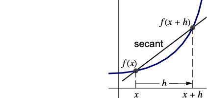
gives the difference quotient ![]() .
.
DifferenceQuotient[f,{x,n,h}]
gives a multiple difference quotient with step h.
DifferenceQuotient[f,{x1,n1,h1},{x2,n2,h2},…]
computes the partial difference quotient with respect to x1,x2,….
Details and Options
- DifferenceQuotient gives the slope of the secant line joining two nearby points on a curve.
- DifferenceQuotient[f,{x,n,h}] is equivalent to DifferenceDelta[f,{x,n,h}]/
 .
. - DifferenceQuotient[f,…,Assumptions->assum] uses the assumptions assum in the course of computing difference quotients.
Examples
open all close allBasic Examples (1)
Compute the difference quotient for a function:
dq = DifferenceQuotient[x Sin[x], {x, h}]Obtain the limit as h approaches 0:
Limit[%, h -> 0]This limit is the derivative of the function:
der = D[x Sin[x], x]Plot[{der, dq /. {h -> 0.5}, dq /. {h -> 0.3}}, {x, 0, 2π}]Scope (16)
Basic Uses (4)
Compute a forward difference quotient with step h:
DifferenceQuotient[f[x], {x, h}]DifferenceQuotient[f[x], {x, -h}]Symmetric difference quotient:
DifferenceQuotient[f[x - h], {x, 2h}]Compute the second difference quotient with step h:
DifferenceQuotient[f[x], {x, 2, h}]DifferenceQuotient[f[x], {x, 3, h}]Partial difference quotient with steps r and s:
DifferenceQuotient[f[x, y], {x, r}, {y, s}]DifferenceQuotient threads over lists:
DifferenceQuotient[{f[x], g[x]}, {x, h}]Univariate Difference Quotients (8)
DifferenceQuotient of a constant is 0:
DifferenceQuotient[c, {x, h}]DifferenceQuotient of a polynomial function is a polynomial function:
DifferenceQuotient[x ^ 3, {x, h}]Each successive difference quotient will lower the degree in x by one:
Table[DifferenceQuotient[x ^ 4, {x, n, h}], {n, 4}]DifferenceQuotient[(x + 1) / (x + 3), {x, h}]Difference quotients of rational functions will stay as rational functions:
Table[DifferenceQuotient[(x + 1) / (x + 3), {x, n, h}], {n, 2}]DifferenceQuotient[Sin[x], {x, h}]DifferenceQuotient[Cos[2x], {x, h}]Table[DifferenceQuotient[a ^ x, {x, n, h}], {n, 3}]DifferenceQuotient[(x ^ 2 + x + 1)2 ^ x, {x, h}]Difference quotients of PolyGamma with an integer step are rational functions:
Block[{h = 3}, Table[DifferenceQuotient[PolyGamma[n, x], {x, h}], {n, 0, 3}]]Similarly for HarmonicNumber and Zeta:
DifferenceQuotient[HarmonicNumber [x, 2], {x, 3}]DifferenceQuotient[Zeta [2, x], {x, 3}]FactorialPower with step h has a simple difference quotient for a matching step h:
DifferenceQuotient[FactorialPower[x, n, h], {x, h}]Multivariate Difference Quotients (4)
DifferenceQuotient of a multivariate polynomial function is a polynomial function:
DifferenceQuotient[x ^ 3 y ^ 2 + 5 x y + 11, {x, h}, {y, k}]Difference quotients of multivariate rational functions will stay as rational functions:
DifferenceQuotient[(x + y + 1) / (((x ^ 2 + 3)(y + 5))), {x, h}, {y, k}]Higher-order quotients will tend to grow in size:
DifferenceQuotient[(x + y + 1) / (((x ^ 2 + 3)(y + 5))), {x, 2, h}, {y, 2, k}]DifferenceQuotient of multivariate functions depending on a subset of the variables are 0:
DifferenceQuotient[f[x], {x, h}, {y, k}]DifferenceQuotient[ g[y], {x, h}, {y, k}]DifferenceQuotient[ h[x, y], {x, h}, {y, k}, {z, p}]DifferenceQuotient for a product of univariate functions:
DifferenceQuotient[f[x] g[y], {x, h}, {y, k}]This is equal to the product of the individual difference quotients:
DifferenceQuotient[f[x], {x, h}]DifferenceQuotient[ g[y], {y, k}]Options (1)
Assumptions (1)
Specify assumptions on the variable x and the step h to obtain simpler results:
DifferenceQuotient[Abs[x], {x, h}]DifferenceQuotient[Abs[x], {x, h}, Assumptions -> x > 0 && h > 0]DifferenceQuotient[Abs[x], {x, h}, Assumptions -> x < 0 && h < 0]Applications (10)
Derivatives from First Principles (3)
Compute the derivative of a polynomial from first principles:
f[x_] := x ^ 2 + 5x + 7Limit[DifferenceQuotient[f[x], {x, h}], h -> 0]Compute the derivative using D:
f'[x]f[x_] := E ^ (a x)Limit[DifferenceQuotient[f[x], {x, h}], h -> 0]f'[x]f[x_] := Sin[2x + 1]Limit[DifferenceQuotient[f[x], {x, h}], h -> 0]f'[x]Compute the second derivative for a power function:
f[x_] := x ^ nLimit[DifferenceQuotient[f[x], {x, 2, h}], h -> 0]f''[x]Third derivative for a power tower:
f[x_] := x ^ xLimit[DifferenceQuotient[f[x], {x, 3, h}], h -> 0]f'''[x]//SimplifyCompute the partial derivative with respect to x for a function of two variables:
f[x_, y_] := Cos[x ^ 2 + E ^ (-y)]Plot3D[f[x, y], {x, -2, 2}, {y, -1, 1}]Limit[DifferenceQuotient[f[x, y], {x, h}], h -> 0]D[f[x, y], x]//SimplifyPartial derivative with respect to y:
Limit[DifferenceQuotient[f[x, y], {y, k}], k -> 0]D[f[x, y], y]Limit[Limit[DifferenceQuotient[f[x, y], {x, h}, {y, k}], h -> 0], k -> 0]D[f[x, y], x, y]Approximate Derivatives (3)
Approximate the derivative at a point using DifferenceQuotient:
f[x_] := 2 x^3 - 15 x^2 + 33 x - 20Plot[f[x], {x, 0, 5}]f'[2.57]Approximation given by DifferenceQuotient:
DifferenceQuotient[f[x], {x, 0.01}] /. {x -> 2.57}Approximate the derivative of a function using various difference quotients:
f[x_] := Sin[E ^ x]Plot[f[x], {x, 0, π}]f'[2]N[%]Use forward difference quotients to obtain an approximation:
hvals = {0.1, 0.01, 0.0001, 0.0001};fd = Table[DifferenceQuotient[f[x], {x, h}], {h, hvals}] /. {x -> 2}Backward difference quotients:
bd = Table[DifferenceQuotient[f[x], {x, -h}], {h, hvals}] /. {x -> 2}Symmetric difference quotients:
Table[DifferenceQuotient[f[x - h], {x, 2h}], {h, {0.1, 0.01, 0.0001, 0.0001}}] /. {x -> 2}Approximate the partial derivatives at a point using DifferenceQuotient:
f[x_, y_] := Sin[x + y]Cos[ 3y]Plot3D[f[x, y], {x, 0, 5}, {y, 0, 5}]{D[f[x, y], {x, 2}], D[f[x, y], x, y], D[f[x, y], {y, 2}]} /. {x -> 2.3, y -> 3.8}{DifferenceQuotient[f[x, y], {x, 2, h}], DifferenceQuotient[f[x, y], {x, h}, {y, k}], DifferenceQuotient[f[x, y], {y, 2, k}]} /. {x -> 2.3, y -> 3.8, h -> 0.001, k -> 0.002}Differential Equations (3)
Discretize a differential equation using forward differences:
deqn = {y'[x] == 2x - y[x], y[0] == 5};reqn = {DifferenceQuotient[y[x], {x, 1 / 10}] == 2x - y[x], y[0] == 5}//SimplifySolve the differential equation using DSolveValue:
dsol = DSolveValue[deqn, y[x], x]Plot[dsol, {x, 0, 5}]Solve the difference equation using RSolveValue:
rsol = RSolveValue[reqn, y[x], x]//SimplifyCompare the exact and approximate solutions:
Table[dsol, {x, 0., 5}]Table[rsol, {x, 0., 5}]Discretize a differential equation using backward differences:
deqn = {y'[x] == 4 - 3y[x], y[0] == 5};reqn = {DifferenceQuotient[y[x], {x, -1 / 10}] == 4 - 3y[x], y[0] == 5}//SimplifySolve the differential equation using DSolveValue:
dsol = DSolveValue[deqn, y[x], x]Plot[dsol, {x, 0, 5}]Solve the difference equation using RSolveValue:
rsol = RSolveValue[reqn, y[x], x]//SimplifyCompare the exact and approximate solutions:
Table[dsol, {x, 0., 5}]Table[rsol, {x, 0., 5}]Discretize a differential equation using symbolic differences:
deqn = {y'[x] == x - 3y[x], y[0] == 1};reqn = {DifferenceQuotient[y[x], {x, h}] == x - 3y[x], y[0] == 1}//SimplifySolve the differential equation using DSolveValue:
dsol = DSolveValue[deqn, y[x], x]//SimplifyPlot[dsol, {x, 0, 5}]Solve the difference equation using RSolveValue:
rsol[h_] = RSolveValue[reqn, y[x], x]Compare the exact and approximate solutions using forward and backward differences:
Table[{dsol, rsol[0.1], rsol[-0.1]}, {x, 0., 5}]//TableFormObtain the exact solution as a limit of the approximate solution:
Limit[rsol[h], h -> 0]//FullSimplifyExtrapolation (1)
Richardson extrapolation is a method for sequence acceleration that can be used to improve the rate of convergence of a sequence a[h], which depends on a parameter h. Apply Richardson extrapolation to accelerate the convergence of DifferenceQuotient to the derivative of a function f[x] using the sequence a[x,h], which is defined by:
a[x_, h_] = DifferenceQuotient[f[x], {x, h}]Set up a scheme for Richardson extrapolation:
r[x_, h_, k_] = (k ^ 2 a[x, h] - a[x, k h]) / (k ^ 2 - 1)//Simplifyf[x_] := x Sin[E ^ (x)]Compute the derivative at a point:
f'[3.4]Approximation given by DifferenceQuotient:
a[3.4, 0.001]Richardson extrapolation improves the derivative approximation:
Table[r[3.4, 0.001, k], {k, {0.5, 0.3, 0.0001}}]Properties & Relations (6)
DifferenceQuotient gives the slope of the secant line joining two nearby points on a curve:
f[x_] := x ^ 3 + 2x - 5diffquotient = DifferenceQuotient[f[x], {x, h}]% /. {x -> 3, h -> 2}secantslope = (f[5] - f[3]) / 2Show[Plot[f[x], {x, 1, 6}], Graphics[{Red, Line[{{2.5, 2.5}, {5.5, 155.5}}]}]]The Limit of DifferenceQuotient is the derivative D:
DifferenceQuotient[f[x], {x, h}]Limit[%, h -> 0, Analytic -> True]An iterated Limit of a multiple difference quotient gives a mixed partial derivative:
DifferenceQuotient[f[x, y], {x, r}, {y, s}]Limit[Limit[%, r -> 0, Analytic -> True], s -> 0, Analytic -> True]DifferenceQuotient is related to DifferenceDelta as ![]() :
:
DifferenceQuotient[f[x], {x, h}] == DifferenceDelta[f[x], {x, 1, h}] / h//SimplifyTable[DifferenceQuotient[f[x], {x, n, h}] == DifferenceDelta[f[x], {x, n, h}] / h ^ n//Simplify, {n, 4}]//SimplifyDifferenceQuotient is related to DiscreteShift as ![]() :
:
DifferenceQuotient[f[x], {x, h}] == (DiscreteShift[f[x], {x, 1, h}] - f[x]) / h//SimplifyDifferenceQuotient is a linear operator:
DifferenceQuotient[f[x] + g[x], {x, h}] == DifferenceQuotient[f[x], {x, h}] + DifferenceQuotient[g[x], {x, h}]//TogetherDifferenceQuotient[c f[x], {x, h}] == c DifferenceQuotient[f[x], {x, h}]//TogetherInteractive Examples (1)
The function ![]() parametrizes the secant line between
parametrizes the secant line between ![]() and
and ![]() :
:
f[x_] = 10 Exp[-(x^2 - x/4)] Sin[2 x];g[h_, b_][x_] = f[b] + (DifferenceQuotient[f[x], {x, h}] /. (x -> b)) (x - b);Visualize how the secant line changes over the function, but at every point becomes tangent as ![]() :
:
Manipulate[
	Plot[{f[x], g[h, b][x]}, {x, -3, 3}, PlotRange -> 12, Epilog -> {AbsolutePointSize[7], Point[{{b, f[b]}, {b + h, f[b + h]}}]}], {{b, 0}, -2, 2, Appearance -> "Labeled"}, {{h, 1}, -1, 1, Appearance -> "Labeled"}, SaveDefinitions -> True]
Neat Examples (1)
Create a table of common difference quotients:
flist = {1, x, x ^ 2, x ^ 3, 1 / x, Sin[x], Cos[x], Sinh[x], Cosh[x], a ^ (x)};Grid[Transpose[{flist, DifferenceQuotient[flist, {x, h}]}], Dividers -> All, Spacings -> {4, 2}, Background -> StandardBlue, BaseStyle -> {FontFamily -> Times, FontSize -> 13}]//TraditionalFormText
Wolfram Research (2016), DifferenceQuotient, Wolfram Language function, https://reference.wolfram.com/language/ref/DifferenceQuotient.html.
CMS
Wolfram Language. 2016. "DifferenceQuotient." Wolfram Language & System Documentation Center. Wolfram Research. https://reference.wolfram.com/language/ref/DifferenceQuotient.html.
APA
Wolfram Language. (2016). DifferenceQuotient. Wolfram Language & System Documentation Center. Retrieved from https://reference.wolfram.com/language/ref/DifferenceQuotient.html