GradientOrientationFilter[data,r]
gives the local orientation parallel to the gradient of data, computed using discrete derivatives of a Gaussian of pixel radius r, returning values between ![]() and
and ![]() .
.


GradientOrientationFilter
GradientOrientationFilter[data,r]
gives the local orientation parallel to the gradient of data, computed using discrete derivatives of a Gaussian of pixel radius r, returning values between ![]() and
and ![]() .
.
GradientOrientationFilter[data,{r,σ}]
uses a Gaussian with standard deviation σ.
Details and Options
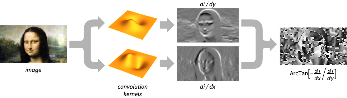
- GradientOrientationFilter is used to obtain the orientation of rapid-intensity change for applications such as texture and fingerprint analysis, as well as object detection and recognition.
- The data can be any of the following:
-
list arbitrary-rank numerical array image arbitrary Image or Image3D object - GradientOrientationFilter[data,r] uses standard deviation
 .
. - GradientOrientationFilter[data,…] returns the orientation as hyperspherical polar coordinate angles. For data arrays of dimensions
 , for
, for  , the resulting array will be of dimensions
  . The
. The  tuples in the resulting array denote the
  -spherical angles.
 - By default, defined angles are returned in the interval
 and the value
  is used for undefined orientation angles.
 - For a single channel image and for data, the gradient
 at a pixel position is approximated using discrete derivatives of Gaussians in each dimension.
 - For multichannel images, define the Jacobian matrix
 to be
to be  , where
  is the gradient for channel
  . The orientation is based on the direction of the eigenvector of
  that has the largest magnitude eigenvalue. This is the direction that maximizes the variation of pixel values.
 - For data arrays with
 dimensions, a coordinate system that corresponds to Part indices is assumed such that a coordinate {x1,…,xn} corresponds to data[[x1,…,xn]]. For images, the filter is effectively applied to ImageData[image].
 - In 1D, the orientation for nonzero gradients is always {0}, and undefined otherwise.
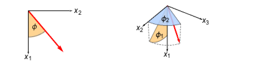
- In 2D, the orientation is the angle
 such that
  is a unit vector parallel to
  .
. - In 3D, the orientation is represented by the angles
 such that
  is a unit vector parallel to the computed gradient.
 - For
 -dimensional data with
  , the orientation is given by angles
  such that
  is a unit vector in the direction of the computed gradient.
 - GradientOrientationFilter[image,…] always returns a single-channel image for 2D images and a two-channel image for 3D images. The result is of the same dimensions as image.
- The following options can be specified:
-
Method Automatic convolution kernel Padding "Fixed" padding method WorkingPrecision Automatic the precision to use - The following suboptions can be given to Method:
-
"DerivativeKernel" "Bessel" convolution kernel "UndefinedOrientationValue" 
return value when orientation is undefined - Possible settings for "DerivativeKernel" include:
-
"Bessel" standardized Bessel derivative kernel, used for Canny edge detection "Gaussian" standardized Gaussian derivative kernel, used for Canny edge detection "ShenCastan" first-order derivatives of exponentials "Sobel" binomial generalizations of the Sobel edge-detection kernels {kernel1,kernel2,…} explicit kernels specified for each dimension - With a setting Padding->None, GradientOrientationFilter[data,…] normally gives an array or image smaller than data.
Examples
open all close allBasic Examples (3)
Gradient orientation of a multichannel image:
GradientOrientationFilter[[image], 4]//ImageAdjustGradient orientation of a 3D image:
GradientOrientationFilter[[image], 2]Gradient orientation filter of a 2D array:
GradientOrientationFilter[(| | | | | |
| - | - | - | - | - |
| 0 | 0 | 1 | 0 | 0 |
| 0 | 1 | 1 | 1 | 0 |
| 1 | 1 | 1 | 1 | 1 |
| 0 | 1 | 1 | 1 | 0 |
| 0 | 0 | 1 | 0 | 0 |), 1]//MatrixFormScope (7)
Data (5)
Gradient orientation of a vector:
GradientOrientationFilter[{1, 1, 0, 1, 0, 1, 1}, 1]Compute gradient orientation symbolically:
GradientOrientationFilter[{{a, b}, {a, b}}, 1]//SimplifyGradient orientation of a binary image:
GradientOrientationFilter[[image], 1]Gradient orientation of a grayscale image:
GradientOrientationFilter[[image], 11]Gradient orientation of a diamond-shaped object:
GradientOrientationFilter[[image], 2]Parameters (2)
Options (8)
Padding (3)
By default, a "Fixed" padding is used:
GradientOrientationFilter[[image], 5]//ImageAdjustGradientOrientationFilter[[image], 5, Padding -> "Periodic"]//ImageAdjustPadding->None normally returns an image smaller than the input image:
GradientOrientationFilter[[image], {19, 3}, Padding -> None]Method (2)
By default, the "Bessel" kernel is used to compute the gradient derivatives:
b = GradientOrientationFilter[[image], 2]Use the "ShenCastan" derivative kernel:
s = GradientOrientationFilter[[image], 2, Method -> "ShenCastan"]The difference between the two methods:
b - sSpecify the value for undefined orientation:
GradientOrientationFilter[{1, 1, 0, 1}, 1, Method -> {"UndefinedOrientationValue" -> None}]WorkingPrecision (3)
MachinePrecision is by default used with integer arrays:
GradientOrientationFilter[{1, 1, 0, 1, 0, 1, 1}, 1]Perform exact computation instead:
GradientOrientationFilter[{1, 1, 0, 1, 0, 1, 1}, 1, WorkingPrecision -> ∞]With real arrays, the precision of the input is used by default:
GradientOrientationFilter[N[{1, 1, 0, 1, 0, 1, 1}, 2], 1]WorkingPrecision is ignored when filtering images:
GradientOrientationFilter[[image], 5, WorkingPrecision -> Infinity]An image of a real type is always returned:
ImageType[%]Applications (5)
Identify the dominant orientations in a noisy image:
img = [image];
o = Flatten@ImageData@GradientOrientationFilter[img, 3];
w = Flatten@ImageData@GradientFilter[img, 3];
Compute and visualize the histogram distribution of weighted orientations:
𝒜 = WeightedData[o, w];
𝒟 = HistogramDistribution[𝒜];
Plot[PDF[𝒟, x], {x, -π / 2, π / 2}, Filling -> Axis, PlotRange -> All, Ticks -> {Range[-π / 2, π / 2, π / 4]}]
Compute the histogram of oriented gradient (HOG) for an image, where each pixel casts a vote weighted by its gradient magnitude in the bin corresponding to its local orientation:
HOG[img_, nbins_] :=
	Module[{mag, ori, mat},
	mag = GradientFilter[img, 1];
	ori = GradientOrientationFilter[img, 1, Method -> {"UndefinedOrientationValue" -> 0}];
	mat = ImageCooccurrence[{mag, ImageAdjust[ori]},
	nbins, {{1}}];
	BarChart[Total[mat * Range[0, 1 - 1 / nbins, 1 / nbins]], ChartLabels -> Join[{-(π/2)}, Table["", {nbins - 2}], {(π/2)}], Axes -> {True, False}]
	];hog = HOG[[image], 10]
Visualize the gradient vectors of an image:
img = [image];
dims = ImageDimensions[img];
dirs = ImageData[GradientOrientationFilter[img, 5]];
magnitudes = ImageData[GradientFilter[img, 5]];
orientations = MapThread[#1{-Sin[#2], Cos[#2]}&, {magnitudes, dirs}, 2];
Show[img, ListVectorPlot[MapIndexed[{{#2[[2]], dims[[2]] - #2[[1]]}, #1}&, orientations, {2}], VectorColorFunction -> (Yellow&), VectorScaling -> Automatic]]
Express orientations in the standard image coordinate system:
i = [image];
orientation = ImageData[GradientOrientationFilter[i, 5]];
orientation = Image@ArcTan[Sin[orientation], -Cos[orientation]];
Visualize the orientation of points on the boundary of the glyph:
pos = RandomChoice[ImageValuePositions[MorphologicalPerimeter[Binarize[i, {0, .5}]], 1], 25];
Show[i, Graphics[Table[{Orange, Arrowheads[{-.02, .02}],
	o = ImageValue[orientation, p];
	Arrow[p + # * {Cos[o], Sin[o]}& /@ {-15, 15}]}, {p, pos}]]]
Show the orientation of features in a fingerprint:
i = [image];r = RidgeFilter[i, 1.5]//ImageAdjustc = (o = GradientOrientationFilter[%, 4])//ImageAdjust//ColorizeImageCompose[i, {c, .5}]Properties & Relations (2)
GradientOrientationFilter is invariant to the size of numbers in the data:
GradientOrientationFilter[(| | | | | |
| - | - | - | - | - |
| 0 | 0 | 1 | 0 | 0 |
| 0 | 1 | 1 | 1 | 0 |
| 1 | 1 | 1 | 1 | 1 |
| 0 | 1 | 1 | 1 | 0 |
| 0 | 0 | 1 | 0 | 0 |), 1]//MatrixFormGradientOrientationFilter[10(| | | | | |
| - | - | - | - | - |
| 0 | 0 | 1 | 0 | 0 |
| 0 | 1 | 1 | 1 | 0 |
| 1 | 1 | 1 | 1 | 1 |
| 0 | 1 | 1 | 1 | 0 |
| 0 | 0 | 1 | 0 | 0 |), 1]//MatrixFormGradient orientation filtering of an image gives a grayscale image of a real type:
GradientOrientationFilter[[image], 3]ImageType[%]Text
Wolfram Research (2012), GradientOrientationFilter, Wolfram Language function, https://reference.wolfram.com/language/ref/GradientOrientationFilter.html (updated 2015).
CMS
Wolfram Language. 2012. "GradientOrientationFilter." Wolfram Language & System Documentation Center. Wolfram Research. Last Modified 2015. https://reference.wolfram.com/language/ref/GradientOrientationFilter.html.
APA
Wolfram Language. (2012). GradientOrientationFilter. Wolfram Language & System Documentation Center. Retrieved from https://reference.wolfram.com/language/ref/GradientOrientationFilter.html