

OrbitalElements
OrbitalElements[body]
returns an association of current orbital elements for the given celestial body in the solar system.
OrbitalElements[body,oelems]
specifies the orbital elements oelems to compute.
OrbitalElements[body,oelems,date]
computes orbital elements for date.
OrbitalElements[ielems,oelems,date]
computes the orbital elements oelems for date from an association ielems of orbital elements.
Details and Options
- Orbital elements describe the geometry and dynamics of the orbital motion of a body around another in the Newtonian two-body approximation.
- Orbital elements are also known as Keplerian elements.
- OrbitalElements is typically used to describe orbits of bodies around other celestial bodies, such as planets around the Sun, moons around planets or artificial satellites around the Earth.
- Orbital elements for entities of these types are given with respect to these frames and origins:
-
"Planet" "EclipticICRS" "Sun" "MinorPlanet" "EclipticICRS" "Sun" "PlanetaryMoon" "EclipticICRS" orbital center, say "Earth" for "Moon" "DeepSpaceProbe" "EclipticICRS" "Sun" "Satellite" "TEME" "Earth" - Orbital elements computed from an association of elements are returned in the same frame as the input.
- Two numbers are needed to describe the shape and size of the orbit, and three are needed to orient it in space. Two more are needed to locate the body along the orbit at a given epoch date. Finally, one more is needed to determine the orbital speed. Therefore, complete orbital information will require at least eight orbital elements, though not every set of eight orbital elements defines an orbit.
- Possible orbital elements describing the shape and size of the orbit include:
-
"Eccentricity" e orbital eccentricity, any non-negative real "SemimajorAxis" a semimajor axis of the orbit "SemiminorAxis" b semiminor axis of the orbit "SemilatusRectum" p semilatus rectum of the orbit "PeriapsisDistance" rp distance from central body to periapsis point "ApoapsisDistance" ra distance from central body to apoapsis point - Possible orbital elements describing the orientation of the orbit in space include:
-
"Inclination" i inclination angle from the reference plane "AscendingNodeLongitude" Ω longitude of the ascending node "PeriapsisArgument" ω angle between ascending node and periapsis "PeriapsisLongitude" ϖ sum of the Ω and ω angles - Possible orbital elements describing the position of the body along the orbit include:
-
"EccentricAnomaly" E eccentric anomaly angle "TrueAnomaly" ν true anomaly angle "MeanAnomaly" M mean anomaly angle "EccentricLongitude" C sum of the ϖ and E angles "TrueLongitude" l sum of the ϖ and ν angles "MeanLongitude" L sum of the ϖ and M angles "LatitudeArgument" u sum of the ω and ν angles - Possible orbital elements determining motion speed include:
-
"StandardGravitationalParameter" GN(m1+m2) product of Newton's gravitational constant and the sum of the masses of the two bodies "MeanMotion" n average angular speed during one orbit "OrbitalPeriod" T period of the orbit "OrbitalEnergy" ϵ specific orbital energy "OrbitalAngularMomentum" h specific orbital angular momentum - Orbital elements whose value is a date include:
-
"Date" t0 date for which the orbital elements are given "PreviousPeriapsisDate" 
date of previous periapsis "NextPeriapsisDate" 
date of next periapsis "PreviousApoapsisDate" 
date of previous apoapsis "NextApoapsisDate" 
date of next apoapsis - Orbital elements related to position and velocity include:
-
"PositionVector" r position vector, measured from central body "VelocityVector" v velocity vector "Radius" r norm of the position vector "Velocity" v norm of the velocity vector "RadialVelocityVector" vr projection of the velocity vector along the position vector "TangentialVelocityVector" vt orthogonal projection of the velocity vector with respect to the position vector "RadialVelocity" vr norm of the radial velocity vector "TangentialVelocity" vt norm of the tangential velocity vector "OrbitTimeSeries" time series of position vectors for an orbit - Other vector-valued orbital elements include:
-
"AngularMomentumVector" h specific angular momentum vector "EccentricityVector" e eccentricity vector "LaplaceRungeLenzVector" R Laplace-Runge-Lenz vector "SemimajorAxisVector" a semimajor axis vector "SemiminorAxisVector" b semiminor axis vector "PeriapsisVector" rp position vector of the periapsis point "AscendingNodeVector" n unitary vector toward the ascending node "ConicCenterVector" c position vector of the conic center - Laskar orbital elements, that do not become singular for circular orbits:
-
"LaskarH" h h=e Sin[ϖ] "LaskarK" k k=e Cos[ϖ] "LaskarP" p p=Sin[i/2]Sin[Ω] "LaskarQ" q q=Sin[i/2]Cos[Ω] - Equinoctial orbital elements, another non-singular set:
-
"EquinoctialF" f f=e Cos[ϖ] "EquinoctialG" g g=e Sin[ϖ] "EquinoctialH" h h=Tan[i/2]Cos[Ω] "EquinoctialK" k k=Tan[i/2]Sin[Ω] - Delaunay action-angle orbital elements:
-
"DelaunayCapitalL" L L=Sqrt[GN(m1+m2)a] "DelaunayCapitalG" G G=Sqrt[GN(m1+m2)p] "DelaunayCapitalH" H H=G Cos[i] - Possible groups of orbital elements include:
-
Automatic selected set of eight orbital elements All all orbital elements in the previous tables - Possible options of OrbitalElements include:
-
Method Automatic source method for computation UnitSystem Automatic unit system for Quantity outputs - Possible unit systems include:
-
Automatic use aus, days and degrees "Dimensionless" or None return numbers in aus, days and radians "SIBase" use meters, seconds and radians "SI" use meters, seconds and degrees "Metric" use kilometers, seconds and degrees "Imperial" use miles, seconds and degrees
Examples
open all close allBasic Examples (4)
Compute orbital elements for Mars at the current moment:
OrbitalElements[Entity["Planet", "Mars"]]Compute the inclination orbital element for Ceres:
OrbitalElements[Entity["MinorPlanet", "Ceres"], "Inclination"]Compute the specified orbital elements for Ceres:
OrbitalElements[Entity["MinorPlanet", "Ceres"], {"Inclination", "SemimajorAxis"}]Compute orbital elements for Neptune on a given date:
OrbitalElements[Entity["Planet", "Neptune"], Automatic, DateObject[{2026, 1, 1, 0, 0, 0}, TimeSystem -> "TDB"]]Given a valid set of orbital elements, find the values of other elements:
ielems = <|"PeriapsisDistance" -> Quantity[1.5, "AstronomicalUnit"], "Eccentricity" -> 0.1, "Inclination" -> Quantity[3, "AngularDegrees"], "AscendingNodeLongitude" -> Quantity[50, "AngularDegrees"], "PeriapsisArgument" -> Quantity[260, "AngularDegrees"], "MeanAnomaly" -> Quantity[130, "AngularDegrees"], "Date" -> DateObject[{2025, 9, 19, 19, 55, 49.057}, "Instant", "Gregorian", 0., "TDB"], "StandardGravitationalParameter" -> Quantity[0.0003, "AstronomicalUnit"^3/"Days"^2]|>;OrbitalElements[ielems, "TrueAnomaly"]OrbitalElements[ielems, {"PreviousPeriapsisDate", "NextPeriapsisDate"}]Scope (12)
Physics Specifications (6)
Find an element of the orbit of a planet around the Sun, with respect to the "EclipticICRS" frame:
OrbitalElements[Entity["Planet", "Jupiter"], "Inclination"]The planet can also be specified as a string:
OrbitalElements["Jupiter", "Inclination"]Compute an orbital element of the orbit of a planetary system barycenter around the Sun:
OrbitalElements["JupiterBarycenter", "Inclination"]Compute an orbital element of the orbit of a planetary moon around its central planet:
OrbitalElements[Entity["PlanetaryMoon", "Callisto"], "Eccentricity"]The moon can also be specified as a string:
OrbitalElements["Callisto", "Eccentricity"]Find an orbital element of the orbit of a satellite around the Earth, with respect to the "TEME" frame:
OrbitalElements[Entity["Satellite", "25544"], "Inclination"]Compute an orbital element from a complete set of orbital elements, with respect to an inertial frame:
oes = <|"PeriapsisDistance" -> Quantity[1.4, "AstronomicalUnit"], "Eccentricity" -> 0.1, "Inclination" -> Quantity[2.5, "AngularDegrees"], "AscendingNodeLongitude" -> Quantity[50, "AngularDegrees"], "PeriapsisArgument" -> Quantity[280, "AngularDegrees"], "MeanAnomaly" -> Quantity[40, "AngularDegrees"], "Date" -> DateObject[{2000, 1, 1, 0, 0, 0}], "StandardGravitationalParameter" -> Quantity[0.0003, "AstronomicalUnit"^3/"Days"^2]|>;This is the position vector of the orbiting body at the same date given by the input orbital elements:
OrbitalElements[oes, "PositionVector"]Compute orbital elements for a hyperbolic orbit, with eccentricity larger than 1:
oes = <|"PeriapsisDistance" -> Quantity[1.4, "AstronomicalUnit"], "Eccentricity" -> 1.3, "Inclination" -> Quantity[2.5, "AngularDegrees"], "AscendingNodeLongitude" -> Quantity[50, "AngularDegrees"], "PeriapsisArgument" -> Quantity[280, "AngularDegrees"], "MeanAnomaly" -> Quantity[40, "AngularDegrees"], "Date" -> DateObject[{2000, 1, 1, 0, 0, 0}], "StandardGravitationalParameter" -> Quantity[0.0003, "AstronomicalUnit"^3/"Days"^2]|>;This is the position vector of the orbiting body at the same date given by the input orbital elements:
OrbitalElements[oes, "PositionVector"]The semimajor axis of a hyperbolic orbit is negative:
OrbitalElements[oes, "SemimajorAxis"]Orbital Elements (4)
By default, OrbitalElements returns a complete set of orbital elements:
OrbitalElements[Entity["Planet", "Neptune"]]This is equivalent to specifying Automatic in the second argument:
OrbitalElements[Entity["Planet", "Neptune"], Automatic]Compute a particular orbital element:
OrbitalElements[Entity["MinorPlanet", "Pluto"], "Eccentricity"]Compute several orbital elements:
OrbitalElements[Entity["MinorPlanet", "Pluto"], {"SemimajorAxis", "SemiminorAxis"}]Compute all available orbital elements for Mars at the current moment:
oes = OrbitalElements[Entity["Planet", "Mars"], All]Apart from numbers and dates, there are Quantity results of these possible units:
DeleteDuplicates[QuantityUnit /@ Cases[oes, _Quantity, Infinity]]Temporal Propagation (2)
Compute orbital elements for the Earth now and in one year's time:
now = NownextYear = now + Quantity[1, "Years"]These are osculating orbital elements corresponding to the given dates, computed directly from NASA's precise ephemerides:
oesNow = OrbitalElements["Earth", Automatic, now]oesNextYear = OrbitalElements["Earth", Automatic, nextYear]Compute the Keplerian prediction of where the Earth will be next year using the current orbital elements:
approx = OrbitalElements[oesNow, Automatic, nextYear]The difference is substantial because the orbit of the Earth is affected by the gravitational pull of the Moon:
oesNextYear - approxThe difference in positions is large, of the order of the Earth-Moon distance:
OrbitalElements[oesNextYear, "PositionVector"] - OrbitalElements[approx, "PositionVector"]UnitConvert[Norm[%], "Kilometers"]Compute orbital elements for the Earth-Moon barycenter (EMB) now and in one year's time:
now = NownextYear = now + Quantity[1, "Years"]oesNow = OrbitalElements["EMB", Automatic, now]oesNextYear = OrbitalElements["EMB", Automatic, nextYear]Compute the Keplerian prediction of where the EMB will be in a year using the current orbital elements:
approx = OrbitalElements[oesNow, Automatic, nextYear]This is the difference of orbital elements:
oesNextYear - approxThe difference in positions is not very large, about one Earth radius in size:
OrbitalElements[oesNextYear, "PositionVector"] - OrbitalElements[approx, "PositionVector"]UnitConvert[Norm[%], "Kilometers"]Options (9)
Method (4)
By default, OrbitalElements computes results based on the NASA ephemeris DE441:
OrbitalElements["Mars"]OrbitalElements["Mars", Method -> Automatic]Use the "VSOP87" ephemeris to compute orbital elements:
OrbitalElements["Mars", Method -> "VSOP87"]Use the "SecularVSOP2013" ephemeris to compute orbital elements:
OrbitalElements["Mars", Method -> "SecularVSOP2013"]Compare the results from different ephemeris sources, for a period of 100 years:
dates = DateRange[DateObject[{2000, 1, 1}], DateObject[{2100, 1, 1}], Quantity[1, "Weeks"]];nasa = TimeSeries@Transpose[{dates, OrbitalElements["Venus", "Eccentricity", #]& /@ dates}];vsop87 = TimeSeries@Transpose[{dates, OrbitalElements["Venus", "Eccentricity", #, Method -> "VSOP87"]& /@ dates}];secular = TimeSeries@Transpose[{dates, OrbitalElements["Venus", "Eccentricity", #, Method -> "SecularVSOP2013"]& /@ dates}];The secular results are effectively an average in time:
DateListPlot[{vsop87, secular}]The results from VSOP87 are close to those of NASA for times close to year 2000:
DateListPlot[vsop87 - nasa]UnitSystem (5)
By default, OrbitalElements returns Quantity outputs in aus, days and degrees:
OrbitalElements["Mars"]OrbitalElements["Mars", UnitSystem -> Automatic]Use the "SIBase" unit system to return outputs in meters, seconds and radians:
OrbitalElements["Mars", UnitSystem -> "SIBase"]Use the "SI" unit system to return outputs in meters, seconds and degrees:
OrbitalElements["Mars", UnitSystem -> "SI"]Use the "Metric" unit system to return outputs in kilometers, seconds and degrees:
OrbitalElements["Mars", UnitSystem -> "Metric"]Use the "Imperial" unit system to return outputs in miles, seconds and degrees:
OrbitalElements["Mars", UnitSystem -> "Imperial"]Applications (5)
Show the orbits of the planets around the Sun:
Graphics3D[OrbitalElements[EntityClass["Planet", All], "OrbitLine"]]Compute approximate orbits for this number of moons around Jupiter:
Length[moons = OrbitalElements[EntityClass["PlanetaryMoon", "JupiterMoon"], "OrbitLine"]//DeleteMissing]Show the orbits around Jupiter, in astronomical units of length:
Graphics3D[moons, Axes -> True]Zoom in to show the inner moons:
Show[%, PlotRange -> 0.2]Zoom even more to show the closest moons, including the Galilean moons:
Show[%, PlotRange -> 0.02]Compute unit normals to the orbital planes of the solar system planets:
planets = EntityList["Planet"]normals = OrbitalElements[planets, "AngularMomentumVector"]They are approximately parallel but differ by a few degrees:
TableForm[Re@Outer[VectorAngle, normals, normals, 1] / Degree, TableHeadings -> {planets, planets}]The largest angle of about 7 degrees corresponds to the planets Mercury and Neptune:
Max[%]Find the date of the first solar eclipse in 2026:
date = SolarEclipse[{2026}]It is an eclipse that will occur near the lunar ascending node:
SolarEclipse[date, "LunarNode"]Find the node direction from Earth's center, as a Cartesian vector in the "EclipticICRS" frame:
OrbitalElements[Entity["PlanetaryMoon", "Moon"], "AscendingNodeVector", date]Convert it to an AstroPosition object in that frame:
anv = AstroPosition[%, {"EclipticICRS", date, "Earth"}, "Cartesian"]Repeat the same operation for the points of the orbit of the Moon:
Values@OrbitalElements[Entity["PlanetaryMoon", "Moon"], "OrbitTimeSeries", date]orbit = AstroPosition[Normal[%], {"EclipticICRS", date, "Earth"}, "Cartesian"]Display together all objects, showing the node as the crossing between the orbits of the Sun and the Moon, with the Moon ascending in ecliptic latitude. The eclipse is not visible from the Earth's center:
Manipulate[AstroGraphics[{StandardPink, Line[orbit], PointSize[Large], Point[anv]}, AstroCenter -> Entity["Star", "Sun"], AstroReferenceFrame -> {"EclipticICRS", date + Quantity[h, "Hours"], "Earth"}, AstroRange -> Quantity[12, "AngularDegrees"]], {h, -10, 20}, SaveDefinitions -> True]Take a deep space probe like Voyager 2:
probe = Entity["DeepSpaceProbe", "Voyager2"];The current part of its orbit is hyperbolic, as shown by the eccentricity being larger than 1:
OrbitalElements[probe]Compute a line of heliocentric coordinates for such approximate orbit:
orbit = OrbitalElements[%, "OrbitLine"];Compute the true orbit of the probe from the date of its launch:
probe["LaunchDate"]trueorbit = Line@Table[AstroPosition[probe, {"EclipticICRS", d, "Sun"}, "Cartesian"]["Data"], {d, % + Quantity[1, "Days"], Now, Quantity[10, "Days"]}];This is the current heliocentric position of the probe, in astronomical units:
pos = OrbitalElements[probe, "PositionVector", UnitSystem -> None]Compare the historical orbit in red with the current hyperbolic fit in black, which agree since the gravitational assist by Neptune:
Graphics3D[{{Opacity[.2], EntityValue["Planet", "OrbitPath"]}, orbit, StandardRed, PointSize[Large], Point[pos], Thick, trueorbit}, Boxed -> False, ViewPoint -> {-2.45, -1.6, 1.8}, PlotRange -> 120, Method -> {"ShrinkWrap" -> True}]Zoom in to see the gravitational assists by Jupiter, Saturn, Uranus and Neptune:
Show[%, PlotRange -> 32]Properties & Relations (1)
OrbitalElements computes osculating orbital elements for the given instant:
body = Entity["Planet", "Neptune"];date0 = Nowoes = OrbitalElements[body, Automatic, date0]Properties at that instant will be precisely computed:
exact[date_] := Quantity[AstroPosition[body, {"EclipticICRS", date, "Sun"}, "Cartesian"]["Data"], "AstronomicalUnit"]OrbitalElements[oes, "PositionVector", date0]% - exact[date0]But the error will generally grow as time passes because the true orbit will be changing:
date = date0 + Quantity[100, "Years"]OrbitalElements[oes, "PositionVector", date]% - exact[date]Show the error growth in astronomical units during a period of 1000 years:
Plot[With[{d = DateObject[{year}, "Instant", "GregorianYear"]}, Norm[OrbitalElements[oes, "PositionVector", d] - exact[d]]], {year, 1500, 2500}]Show the shape of the difference, in the ecliptic frame:
ParametricPlot3D[With[{d = DateObject[{year}, "Instant", "GregorianYear"]}, OrbitalElements[oes, "PositionVector", d] - exact[d]], {year, 1500, 2500}]Interactive Examples (1)
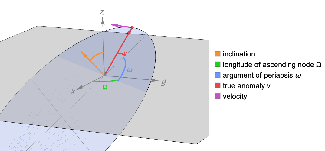
Change the values of the input orbital elements to see how each one affects the resulting orbit:
angle[z_, x_, a_, scale_, text_] := With[{n = 50, nx = Normalize[x], ny = Normalize[Cross[z, x]], ar = a Degree, s = 0.4scale, p = 0.1}, {color[text], Line@Table[s(Cos[t]nx + Sin[t]ny), {t, Min[0, ar], Max[0, ar], Max[Abs@ar / n, 0.01]}], Text[Style[text, "Bold"], (s + p)(Cos[ar / 2]nx + Sin[ar / 2]ny)]}];
axis[v_, label_] := {AbsoluteThickness[1], Gray, Arrow[{{0, 0, 0}, v}], Text[Style[label, 18], 1.1v]};
color["ν"] = StandardRed;
color["Ω"] = StandardGreen;
color["i"] = StandardOrange;
color["ω"] = StandardBlue;
color["v"] = StandardPurple;
limit[e_] := 180If[e <= 1, 1, ArcTan[Sqrt[(1 + e/-1 + e)] Tanh[(π/2)]] / ((π/2))]
Manipulate[
	Module[{pos, vel, av, bv, cv, nv, hv, pv, ts, ov = {0, 0, 0}, xv = {1, 0, 0}, yv = {0, 1, 0}, zv = {0, 0, 1}, date = Now},
	{pos, vel, av, bv, cv, nv, hv, pv, ts} = Lookup[OrbitalElements[<|"PeriapsisDistance" -> rp, "Eccentricity" -> e, "Inclination" -> i Degree, "PeriapsisArgument" -> ω Degree, "AscendingNodeLongitude" -> Ω Degree, "TrueAnomaly" -> ν Degree, "Date" -> date, "StandardGravitationalParameter" -> 0.0003|>, All, date, UnitSystem -> "Dimensionless"], {"PositionVector", "VelocityVector", "SemimajorAxisVector", "SemiminorAxisVector", "ConicCenterVector", "AscendingNodeVector", "AngularMomentumVector", "PeriapsisVector", "OrbitTimeSeries"}];
	Graphics3D[{
	Thick, Arrowheads[Medium],
	{Opacity[0.5], GrayLevel[0.7], InfinitePlane[ov, {xv, yv}]},
	{Thin, Gray, If[e == 1, HalfLine[pv, -pv], Line[{{cv - av, If[e < 1, cv + av, ov]}, {cv - bv, cv + bv}}]]},
	{axis[rp xv, "𝓍"], axis[rp yv, "𝓎"], axis[rp zv, "𝓏"]},
	{EdgeForm[Black], Opacity[0.15], RGBColor[0, .25, 1], Polygon[Normal@Values@ts]},
	{color["v"], Arrow[{pos, pos + 30vel}]},
	{color["ν"], Arrow[{ov, pos}], Sphere[pos, rp / 40]},
	{color["i"], Arrow[{ov, 30hv}]},
	{angle[zv, xv, Ω, rp, "Ω"], angle[hv, nv, ω, 1.1rp, "ω"], angle[hv, pv, ν, 1.2rp, "ν"], angle[nv, zv, i, rp, "i"]}
	},
	PlotRange -> 3, ViewPoint -> {3.45, 1.85, 1.}, ViewVertical -> {0.22, 0.15, 1}, RotationAction -> "Clip", ViewAngle -> (π/30), Boxed -> False, Axes -> False, Lighting -> "Neutral", ImageSize -> {600, 400}, Method -> {"EdgeDepthOffset" -> False}]
	],
	{{rp, 1, "periapsis distance (rp)"}, .1, 5, Appearance -> "Labeled"},
	{{e, 0.5, "eccentricity (e)"}, 0, 2, Appearance -> "Labeled"},
	{{i, 42, Style["inclination (i)", color["i"], Bold]}, 0, 180, Appearance -> "Labeled"},
	{{Ω, 57, Style["longitude of ascending node (Ω)", color["Ω"], Bold]}, 0, 360, Appearance -> "Labeled"},
	{{ω, 77, Style["argument of periapsis (ω)", color["ω"], Bold]}, 0, 360, Appearance -> "Labeled"},
	{{ν, 30, Style["true anomaly (𝓋)", color["ν"], Bold]}, -limit[e], limit[e], Appearance -> "Labeled"},
	SaveDefinitions -> True
	]
Neat Examples (1)
Find the list of GPS satellites:
SatelliteData[EntityClass["Satellite", "GPS"]]Compute current orbital elements for them:
oes = OrbitalElements[EntityClass["Satellite", "GPS"]];Build approximate orbits around the Earth:
orbits = OrbitalElements[oes, "OrbitLine"];Model the Earth as a blue sphere:
earth = {StandardBlue, Sphere[{0, 0, 0}, QuantityMagnitude[Entity["Planet", "Earth"]["Radius"], "AstronomicalUnit"]]};Show how the satellites move in space during the next 24 hours:
Manipulate[Graphics3D[{earth, orbits, Red, PointSize[Large], Point[OrbitalElements[oes, "PositionVector", Now + Quantity[h, "Hours"], UnitSystem -> None]]}, ImageSize -> 400], {h, 0, 24}, SaveDefinitions -> True]Text
Wolfram Research (2026), OrbitalElements, Wolfram Language function, https://reference.wolfram.com/language/ref/OrbitalElements.html.
CMS
Wolfram Language. 2026. "OrbitalElements." Wolfram Language & System Documentation Center. Wolfram Research. https://reference.wolfram.com/language/ref/OrbitalElements.html.
APA
Wolfram Language. (2026). OrbitalElements. Wolfram Language & System Documentation Center. Retrieved from https://reference.wolfram.com/language/ref/OrbitalElements.html