

TukeyWindow
TukeyWindow[x]
represents a Tukey window function of x.
TukeyWindow[x,α]
uses the parameter α.
Details
- TukeyWindow, also known as the cosine-tapered window, is a window function typically used in signal processing applications where data needs to be processed in short segments.
- Window functions have a smoothing effect by gradually tapering data values to zero at the ends of each segment.
- TukeyWindow[x,α] is equal to
![ 1 (0<a<1∧a-2 x-1<=0∧a+2 x-1<=0)∨(a=1∧x=0)∨(a<=0∧-1/2<=x<=1/2); 1/2 (cos(2 pi x)+1) a>1∧-1/2<=x<=1/2; 1/2 (cos((2 pi (-a/2+x+1/2))/a)+1) 0<a<=1∧x>=-1/2∧a-2 x-1>0; 1/2 (cos((2 pi (a/2+x-1/2))/a)+1) 0<a<=1∧a+2 x-1>0∧x<=1/2; 0 TemplateBox[{x}, Abs]>1/2;](Files/TukeyWindow.en/2.png " 1 (0<a<1∧a-2 x-1<=0∧a+2 x-1<=0)∨(a=1∧x=0)∨(a<=0∧-1/2<=x<=1/2); 1/2 (cos(2 pi x)+1) a>1∧-1/2<=x<=1/2; 1/2 (cos((2 pi (-a/2+x+1/2))/a)+1) 0<a<=1∧x>=-1/2∧a-2 x-1>0; 1/2 (cos((2 pi (a/2+x-1/2))/a)+1) 0<a<=1∧a+2 x-1>0∧x<=1/2; 0 TemplateBox[{x}, Abs]>1/2;") .
. - TukeyWindow[x] is equivalent to TukeyWindow[x,2/3].
- TukeyWindow automatically threads over lists.
Examples
open all close allBasic Examples (3)
Plot[TukeyWindow[x], {x, -1, 1}]Plot3D[TukeyWindow[x]TukeyWindow[y], {x, -1, 1}, {y, -1, 1}, PlotRange -> All, Exclusions -> None]Extract the continuous function representing the Tukey window:
FunctionExpand[TukeyWindow[x]]FunctionExpand[TukeyWindow[x, α]]Scope (6)
TukeyWindow[.4]Shape of a 1D Tukey window using a specified parameter:
Plot[TukeyWindow[x], {x, -1, 1}]Variation of the shape as a function of the parameter α:
Plot3D[TukeyWindow[x, α], {α, 1 / 3, 1}, {x, -1, 1}]Translated and dilated Tukey window:
Plot[TukeyWindow[(x - 1) / 2], {x, -1, 3}]2D Tukey window with a circular support:
Plot3D[TukeyWindow[Sqrt[x ^ 2 + y ^ 2]], {x, -1, 1}, {y, -1, 1}, PlotRange -> All, Exclusions -> None]Discrete Tukey window of length 15:
ListPlot[Array[TukeyWindow, 15, {-1 / 2, 1 / 2}], Filling -> Axis]Discrete 15×10 2D Tukey window:
ListPointPlot3D[Array[TukeyWindow[#1] TukeyWindow[#2]&, {15, 10}, {{-1 / 2, 1 / 2}}], Filling -> Axis]Applications (3)
Use the Tukey window to diminish the effect of signal partitioning when computing the spectrogram:
Labeled[Spectrogram[\!\(\*AudioBox[""]\), 512, Automatic, #, ImageSize -> 200, FrameTicks -> None], Text[#]]& /@ {TukeyWindow, None}Use a window specification to calculate sample PowerSpectralDensity:
proc = ARMAProcess[1, {.5}, {.3}, 1];
data = RandomFunction[proc, {50}];spec = PowerSpectralDensity[data, w, TukeyWindow];Compare to spectral density calculated without a windowing function:
sd = PowerSpectralDensity[data, w];sd === specThe plot shows that the window smooths the spectral density:
Plot[{sd, spec}, {w, -π, π}, PlotRange -> All, PlotLegends -> {"no window", "with window"}]Compare to the theoretical spectral density of the process:
Plot[{spec, Evaluate@PowerSpectralDensity[proc, w]}, {w, -π, π}, PlotLegends -> {"data", "process"}]Use a window specification for time series estimation:
data = RandomFunction[ARMAProcess[1, {.3}, {.4}, 1], {300}];Specify window for spectral estimator:
EstimatedProcess[data, ARMAProcess[1, 1], ProcessEstimator -> {"SpectralEstimator", "Window" -> TukeyWindow}]Properties & Relations (10)
TukeyWindow[x,1] is equivalent to a Hann window:
Simplify[FunctionExpand[TukeyWindow[x, 1]]] == Simplify[FunctionExpand[HannWindow[x]]]TukeyWindow[x,0] is equivalent to a box window:
Simplify[FunctionExpand[TukeyWindow[x, 0]]] == Simplify[FunctionExpand[DirichletWindow[x]]]TukeyWindow[x,1] is equivalent to a Hann window:
Simplify[FunctionExpand[TukeyWindow[x, 1]]] == Simplify[FunctionExpand[HannWindow[x, 1 / 2]]]Tukey window is a convolution of a unit pulse with a raised cosine:
4 Convolve[UnitBox[y], (1/2)(Cos[4 π y] + 1)UnitBox[2y], y, x] /. x -> 3 / 2 x//PiecewiseExpandPlot[%, {x, -1, 1}]The area under the Tukey window:
area = Integrate[TukeyWindow[x], {x, -∞, ∞}]Normalize to create a window with unit area:
Plot[{TukeyWindow[x], TukeyWindow[x] / area}, {x, -1, 1}, PlotRange -> All]Fourier transform of the Tukey window:
f = FourierTransform[TukeyWindow[x], x, w]Power spectrum of the Tukey window:
LogLinearPlot[20 Log[10, Abs[f]], {w, .1, 80}]Fourier transform of the parametrized Tukey window:
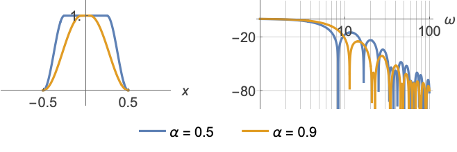
f = FourierTransform[TukeyWindow[x, α], x, ω]//SimplifyVariation of the magnitude spectrum of the Tukey window as a function of the parameter ![]() :
:
Plot3D[Abs@f, {ω, -30, 30}, {α, 0, 2}, PlotRange -> All, Exclusions -> None]Discrete-time Fourier transform of the discrete Tukey window of length 11:
(f = ListFourierSequenceTransform[Array[TukeyWindow, 11, {-1 / 2, 1 / 2}], ω])//Shortf0 = N[f /. ω -> 0]Plot[Abs@f / f0, {ω, 0, π}, PlotRange -> All]Power spectra for three different window lengths:
tab = Table[(f = ListFourierSequenceTransform[Array[TukeyWindow, n, {-1 / 2, 1 / 2}], ω];
f0 = N[f /. ω -> 0];
20Log10[Abs@f / f0]), {n, {5, 15, 45}}];LogLinearPlot[tab, {ω, 0.01, π}, PlotRange -> {5, -40}, PlotLegends -> {5, 15, 45}]Power spectra for three different values of the shape parameter ![]() :
:
tab = Table[(f = ListFourierSequenceTransform[Array[TukeyWindow[#, α]&, 15, {-1 / 2, 1 / 2}], ω];
f0 = N[f /. ω -> 0];
20Log10[Abs@f / f0]), {α, {1 / 3, 2 / 3, 5 / 3}}];LogLinearPlot[tab, {ω, 0.05, π}, PlotRange -> {5, -40}, PlotLegends -> {1 / 3, 2 / 3, 5 / 3}]Possible Issues (1)
2D sampling of Tukey window will use a different parameter for each row of samples when passed as a symbol to Array:
Array[TukeyWindow, {30, 30}, {{-1 / 2, 1 / 2}}]//ListPlot3DArray[TukeyWindow[#1] TukeyWindow[#2]&, {30, 30}, {{-1 / 2, 1 / 2}}]//ListPlot3DText
Wolfram Research (2012), TukeyWindow, Wolfram Language function, https://reference.wolfram.com/language/ref/TukeyWindow.html (updated 2016).
CMS
Wolfram Language. 2012. "TukeyWindow." Wolfram Language & System Documentation Center. Wolfram Research. Last Modified 2016. https://reference.wolfram.com/language/ref/TukeyWindow.html.
APA
Wolfram Language. (2012). TukeyWindow. Wolfram Language & System Documentation Center. Retrieved from https://reference.wolfram.com/language/ref/TukeyWindow.html