"PrincipalComponentsAnalysis" (Machine Learning Method)
"PrincipalComponentsAnalysis" (Machine Learning Method)
- Method for DimensionReduction, DimensionReduce, FeatureSpacePlot and FeatureSpacePlot3D.
- Maps the data into a lower-dimensional space using the principal components analysis method.
Details & Suboptions
- "PrincipalComponentsAnalysis" is a linear dimensionality reduction method. The method projects input data on a linear lower-dimensional space that preserves the maximum variance in the data.
- The "PrincipalComponentsAnalysis" method works for datasets that have a large number of features and large number of examples; however, the learned manifold can only be linear.
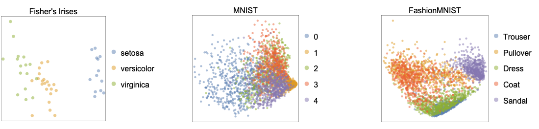
- The following plots show the results of the "PrincipalComponentsAnalysis" method applied to benchmark datasets including Fisher's Irises, MNIST and FashionMNIST:
- "PrincipalComponentsAnalysis" is equivalent to the "Linear" and "LatentSemanticAnalysis" methods when the data is standardized.
Examples
open all close allBasic Examples (1)
Train a linear dimensionality reduction using the "PrincipalComponentsAnalysis" method from a list of vectors:
reducer = DimensionReduction[{{1, 2, 3}, {2, 3, 5}, {3, 5, 8}, {4, 5, 8.5}}, 2, Method -> "PrincipalComponentsAnalysis"]Use the trained reducer on new vectors:
reducer[{{6, 7, 14}, {5, 6, 11}, {1, 3, 9}}]Scope (1)
Dataset Visualization (1)
Load the Fisher Iris dataset from ExampleData:
iris = ExampleData[{"MachineLearning", "FisherIris"}, "Data"];RandomSample[iris, 5]Generate a reducer function using "PrincipalComponentsAnalysis" with the features of each example:
diris = DimensionReduction[iris[[All, 1]], 2, Method -> "PrincipalComponentsAnalysis"]Group the examples by their species:
byspecies = GroupBy[iris, Last -> First];Reduce the dimension of the features:
byspecies = diris /@ byspecies;Visualize the reduced dataset:
ListPlot[Values[byspecies], PlotLegends -> Keys[byspecies]]