

CarlemanLinearize
CarlemanLinearize[sys,spec]
Carleman linearizes the nonlinear state-space model sys according to spec.
Details
- CarlemanLinearize gives an approximation of the infinite order system in which sys is embedded.
- For input-linear systems, the result is bilinear, that is, linear in both the states and inputs. In general, it is linear only in the states.
- Possible values for spec:
-
k approximation order {{e1,…,en}} monomials of the embedding transformation {…,{z1,…,zn}} new state variables {…,z,order} monomial ordering - Possible settings for order are the same as in MonomialList.
- CarlemanLinearize returns a LinearizingTransformationData object that can be used to extract various properties.
- The following properties can be given:
-
"EmbeddingTransformation" {z1->e1,…,zn->en} "TransformedSystem" approximate transformed system {"OriginalSystemController",κ} controller for the original system sys {"OriginalSystemEstimator",ℓ} estimator for the original system sys {"ClosedLoopSystem",κ} closed-loop system of sys with the controller
Examples
open all close allBasic Examples (1)
Carleman linearize a nonlinear system:
𝒞ℒ = CarlemanLinearize[AffineStateSpaceModel[{{E^x}, {{1 + x^2}}, {x}, {{0}}},
{x}, Automatic, {Automatic}, Automatic, SamplingPeriod -> None], 3]tsys = 𝒞ℒ["TransformedSystem"]Design a controller based on the linearized model:
κ = StateFeedbackGains[StateSpaceModel[tsys], {-0.5, -1 + I, -1 - I}]csys = 𝒞ℒ[{"ClosedLoopSystem", κ}]Simulate the closed-loop system:
OutputResponse[csys, 1, {t, 0, 20}];
Plot[%, {t, 0, 1}, PlotRange -> All]
Scope (10)
Basic uses (6)
Carleman linearize an affine system:
𝒞ℒ = CarlemanLinearize[AffineStateSpaceModel[{{x^2}, {{1}}, {x}, {{0}}}, {x},
 Automatic, {Automatic}, Automatic, SamplingPeriod -> None], 4]
The transformed system is bilinear:
𝒞ℒ["TransformedSystem"]SystemsModelLinearity[%]𝒞ℒ["EmbeddingTransformation"]Specify the new variables to use:
𝒞ℒ = CarlemanLinearize[AffineStateSpaceModel[{{x^2}, {{1}}, {x}, {{0}}}, {x},
 Automatic, {Automatic}, Automatic, SamplingPeriod -> None], {4, {Subscript[z, 1], Subscript[z, 2], Subscript[z, 3], Subscript[z, 4]}}]
The results are now in terms of the specified variables:
𝒞ℒ[{"TransformedSystem", "EmbeddingTransformation"}]Specify the terms of the transformation:
𝒞ℒ = CarlemanLinearize[AffineStateSpaceModel[{{x^2}, {{1}}, {x}, {{0}}}, {x},
Automatic, {Automatic}, Automatic, SamplingPeriod -> None], {{x, x^2, x^4, x^7}, {Subscript[z, 1], Subscript[z, 2], Subscript[z, 3], Subscript[z, 4]}}]𝒞ℒ[{"TransformedSystem", "EmbeddingTransformation"}]𝒞ℒ = CarlemanLinearize[AffineStateSpaceModel[{{x^2}, {{1}}, {x}, {{0}}}, {x},
Automatic, {Automatic}, Automatic, SamplingPeriod -> None], {4, {Subscript[z, 1], Subscript[z, 2], Subscript[z, 3], Subscript[z, 4]}, "Lexicographic"}]𝒞ℒ[{"TransformedSystem", "EmbeddingTransformation"}]Directly specify the property:
CarlemanLinearize[AffineStateSpaceModel[{{x^2}, {{1}}, {x}, {{0}}}, {x},
Automatic, {Automatic}, Automatic, SamplingPeriod -> None], 4, "TransformedSystem"]CarlemanLinearize[AffineStateSpaceModel[{{x^2}, {{1}}, {x}, {{0}}}, {x},
Automatic, {Automatic}, Automatic, SamplingPeriod -> None], 4, {"TransformedSystem", "EmbeddingTransformation"}]The linearization of a NonlinearStateSpaceModel:
𝒞ℒ = CarlemanLinearize[NonlinearStateSpaceModel[{{u + u^2 + x^2},
  {x}}, {x}, {u}, {Automatic}, Automatic,
 SamplingPeriod -> None], {4, {Subscript[z, 1], Subscript[z, 2], Subscript[z, 3], Subscript[z, 4]}}]
The transformed system is linear in the states:
𝒞ℒ["TransformedSystem"]SystemsModelLinearity[%]Properties (4)
CarlemanLinearize[AffineStateSpaceModel[{{x^2}, {{1}}, {x}, {{0}}}, {x},
Automatic, {Automatic}, Automatic, SamplingPeriod -> None], 4, "Properties"]𝒞ℒ = CarlemanLinearize[AffineStateSpaceModel[{{x^2}, {{1}}, {x}, {{0}}}, {x},
Automatic, {Automatic}, Automatic, SamplingPeriod -> None], 4];𝒞ℒ["EmbeddingTransformation"]𝒞ℒ["TransformedSystem"]asys = AffineStateSpaceModel[{{x + x^2}, {{1}}, {x}, {{0}}},
{{x, -1}}, Automatic, {Automatic}, Automatic, SamplingPeriod -> None];𝒞ℒ = CarlemanLinearize[asys, {4, {Subscript[z, 1], Subscript[z, 2], Subscript[z, 3], Subscript[z, 4]}}]Design a controller based on the Taylor linearization of the transformed system:
κ = StateFeedbackGains[StateSpaceModel@𝒞ℒ["TransformedSystem"], {-0.5, -1, -2 + I, -2 - I}]The closed-loop system is a composite property:
csys = 𝒞ℒ[{"ClosedLoopSystem", κ}]//Simplifyor = OutputResponse[{csys, -2}, 0, {t, 0, 5}];
Show[p = Plot[or, {t, 0, 5}, PlotRange -> All], PlotRange -> {{0, 0.5}, All}]The controller for the original system:
𝒞ℒ[{"OriginalSystemController", κ}]Plot[𝒞ℒ[{"OriginalSystemController", κ}] /. x -> or, {t, 0, 0.5}, PlotRange -> All]The closed-loop system based on the Taylor linearization design:
csys1 = SystemsModelStateFeedbackConnect[asys, StateFeedbackGains[StateSpaceModel[asys], {-3}]]or1 = OutputResponse[{csys1, -2}, 0, {t, 0, 5}];
p1 = Plot[or1, {t, 0, 5}, PlotRange -> All, PlotStyle -> Dashed]Show[p, p1]Design an estimator using Carleman linearization:
asys = AffineStateSpaceModel[{{-2*x + x^2 - y + y^2,
   x^2 - 2*y}, {{1}, {1}}, {x}, {{0}}},
 {{x, -1}, {y, -1}}, Automatic, {Automatic}, Automatic,
SamplingPeriod -> None];𝒞ℒ = CarlemanLinearize[asys, {2, {Subscript[z, 1], Subscript[z, 2], Subscript[z, 3], Subscript[z, 4], Subscript[z, 5]}}]A set of estimator gains for the transformed system:
ℓ = EstimatorGains[StateSpaceModel@𝒞ℒ["TransformedSystem"], {-3, -4, -5, -6 + 2 I, -6 - 2I}]The estimator for the original system:
estim = 𝒞ℒ[{"OriginalSystemEstimator", ℓ}]The trajectories of the estimated states:
or = OutputResponse[{asys, {-0.2, 0.1}}, 0, {t, 0, 5}];res1 = OutputResponse[SystemsModelDelete[estim, None, 3], Join[{0}, or], {t, 0, 5}];Plot[res1, {t, 0, 5}, PlotRange -> All]The actual state trajectories:
res = StateResponse[{asys, {-0.2, 0.1}}, 0, {t, 0, 5}];Compare the actual and estimated state trajectories:
Plot[Evaluate@Flatten@{res, res1}, {t, 0, 5}, PlotRange -> All, PlotLegends -> {"State 1", "State 2", "Estimated State 1", "Estimated State 2"}]Applications (2)
Design a therapy for HIV-1 infection based on Carleman linearization. The parameters are the decay rate ![]() and production rate
and production rate ![]() of healthy cells, infection rate coefficient
of healthy cells, infection rate coefficient ![]() , and decay rate
, and decay rate ![]() of the virus: »
of the virus: »
pars = {d -> 0.02, s -> 10, θ -> 0.001, μ -> 0.24};The states are the levels of healthy cells ![]() and free virus
and free virus ![]() , and the input is the drug dosage:
, and the input is the drug dosage:
asys = AffineStateSpaceModel[{{s - d*Subscript[x, 1] -
    θ*Subscript[x, 1]*Subscript[x, 2],
   (-μ)*Subscript[x, 2] + θ*Subscript[x, 1]*
     Subscript[x, 2]},
  {{θ*Subscript[x, 1]*Subscript[x, 2]},
   {(-θ)*Subscript[x, 1]*Subscript[x, 2]}}},
 {{Subscript[x, 1], (s - r*μ)/d},
  {Subscript[x, 2], r}},
 {{u, (s*θ - d*μ -
     r*θ*μ)/(θ*
     (s - r*μ))}}, {Automatic, Automatic}, Automatic,
 SamplingPeriod -> None] /. pars
At the target level of 10, a low dosage results in increased virus levels:
sr = StateResponse[asys /. r -> 10, 0.2, {t, 0, 20}];
Table[Plot[sr, {t, 0, 20}], {sr, sr}]
Carleman linearize the system:
𝒞ℒ = CarlemanLinearize[asys /. r -> 10, {{Subscript[x, 1], Subscript[x, 2], Subscript[x, 1]Subscript[x, 2]}}]Design a controller for the linearized, higher-order system:
ssm = StateSpaceModel[𝒞ℒ["TransformedSystem"]];κ = LQRegulatorGains[ssm, {DiagonalMatrix[{0.1, 50, 25}], {{3000}}}]csys = 𝒞ℒ[{"ClosedLoopSystem", κ}]//SimplifyThe controller brings the healthy cell and virus concentrations to the desired levels:
sr = StateResponse[{csys, {370, 14}}, 0, {t, 0, 600}];
Table[Plot[sr, {t, 0, 600}], {sr, sr}]-𝒞ℒ[{"OriginalSystemController", κ}];
Plot[% /. Thread[{Subscript[x, 1], Subscript[x, 2]} -> sr], {t, 0, 600}]Design an estimator using Carleman linearization to estimate the reactant concentration based on the reactor temperature in a continuous stirred-tank reactor (CSTR): »
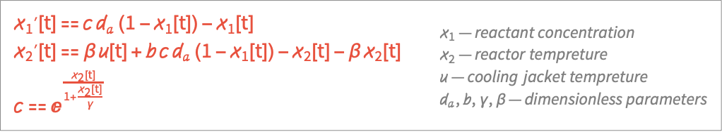
Assemble the model with ![]() as input and
as input and ![]() as states:
as states:
aa = With[{c = (1 - Subscript[x, 1])Exp[Subscript[x, 2] / (1 + Subscript[x, 2] / γ)]}, {-Subscript[x, 1] + Subscript[d, a] c, -Subscript[x, 2] + b Subscript[d, a]c - β Subscript[x, 2]}];
bb = {{0}, {β}};
cc = {Subscript[x, 2]};pars = {β -> 1, Subscript[d, a] -> 1, b -> 1, γ -> 1};sys = AffineStateSpaceModel[{aa, bb, cc}, {Subscript[x, 1], Subscript[x, 2]}] /. parsCarleman linearize the system:
𝒞ℒ = CarlemanLinearize[sys, 4]𝒞ℒ["TransformedSystem"]EstimatorGains[StateSpaceModel[%], -Range[1, 14]//N];estim = 𝒞ℒ[{"OriginalSystemEstimator", %}]Compute the actual reactant concentration:
𝒸 = StateResponse[{sys, {0.5, 3}}, 1, {t, 0, 7}][[1]];
Plot[𝒸, {t, 0, 7}, PlotRange -> All]
Compare the actual and estimated values:
ℴ = OutputResponse[{sys, {0.5, 3}}, 1, {t, 0, 7}];
𝒸ℯ = OutputResponse[estim, Join[{1}, ℴ], {t, 0, 7}][[1]];Plot[{𝒸, 𝒸ℯ}, {t, 0, 7}, PlotLegends -> {"Actual", "Estimated"}, PlotRange -> All]Properties & Relations (1)
Carleman linearization of order 1:
assm = AffineStateSpaceModel[
 {{ω, (g*m*(m + M)*
      Sin[θ])/(l*m^2 + l*m*
       M - l*m^2*Cos[θ]^2) -
    (l*m^2*ω^2*Cos[θ]*Sin[θ])/
     (l*m^2 + l*m*M -
      l*m^2*Cos[θ]^2), v,
   (l^2*m^2*ω^2*Sin[θ])/
     (l*m^2 + l*m*M -
      l*m^2*Cos[θ]^2) -
    (g*l*m^2*Cos[θ]*Sin[θ])/
     (l*m^2 + l*m*M -
      l*m^2*Cos[θ]^2)},
  {{0}, {(-m)*(Cos[θ]/(l*m^2 +
       l*m*M - l*m^2*
        Cos[θ]^2))}, {0},
   {l*(m/(l*m^2 +
       l*m*M - l*m^2*
        Cos[θ]^2))}}, {θ, x}, {{0}, {0}}},
 {θ, ω, x, v}, {{F, 0}},
{θ, x}, Automatic, SamplingPeriod -> None];CarlemanLinearize[assm, 1, "TransformedSystem"]It is equivalent to Taylor linearization:
StateSpaceModel[assm]Text
Wolfram Research (2014), CarlemanLinearize, Wolfram Language function, https://reference.wolfram.com/language/ref/CarlemanLinearize.html.
CMS
Wolfram Language. 2014. "CarlemanLinearize." Wolfram Language & System Documentation Center. Wolfram Research. https://reference.wolfram.com/language/ref/CarlemanLinearize.html.
APA
Wolfram Language. (2014). CarlemanLinearize. Wolfram Language & System Documentation Center. Retrieved from https://reference.wolfram.com/language/ref/CarlemanLinearize.html