

FeedbackLinearize
FeedbackLinearize[asys]
input-output linearizes the AffineStateSpaceModel asys by state transformation and feedback.
FeedbackLinearize[asys,{z,v}]
specifies the new states z and the new control inputs v.
FeedbackLinearize[asys,{z,v},"prop"]
computes the property "prop".
Details and Options
- FeedbackLinearize is also known as exact linearization.
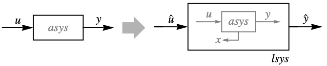
- FeedbackLinearize will construct a linear system lsys from a nonlinear system asys in such a way that you can use linear control design techniques for the linear system lsys to control the nonlinear system asys.
- FeedbackLinearize returns a LinearizingTransformationData object that can be used to extract the properties needed for analysis and design based on feedback linearization.
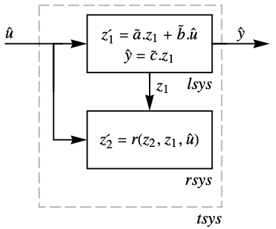
- The transformed system tsys consists of a linear system lsys and possibly a residual system rsys with internal dynamics that need to be stable, but is otherwise not observable.
- Properties related to the transformed system include:
-
"LinearSystem" systems model lsys "ResidualSystem" systems model rsys "TransformedSystem" systems model tsys - By designing a stabilizing controller cs for lsys, the resulting closed-loop system will be stable, provided that the residual system rsys is stable.
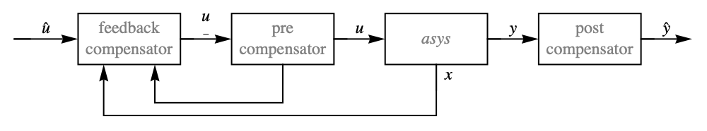
- In order to deploy the controller for the original nonlinear system asys, you need to transform the controller cs to use the original variables.
- Properties related to transforming the controller and estimator to original coordinates:
-
{"OriginalSystemController",cs} controller cs in original coordinates {"OriginalSystemEstimator",es} estimator for  and
and 
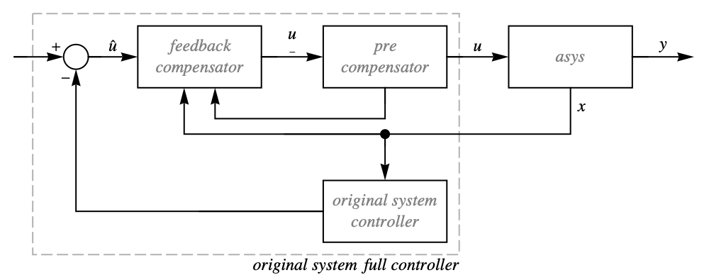
{"ClosedLoopSystem",cs} closed-loop system in original coordinates {"OriginalSystemFullController",cs} systems model of cs in original coordinates - Further detailed properties of feedback linearization are also available and can be used to deploy alternative simulations and implementations of controllers, estimators, etc.
- The system asys
 is connected with a feedback compensator, precompensator, and postcompensator to give a modified system
  , where
  is the modified input,
  is the state vector that consists of
  with possible additional compensator states, and
  is the modified output.
 - The feedback compensator is essentially a transformation between
 and
and  given by
  , where
  is the decoupling matrix.
 - Compensator properties include:
-
"FeedbackCompensator" systems model from  to
to 
"InverseFeedbackCompensator" systems model from  to
to 
"InverseFeedbackTransformation" list of rules 
"DecouplingMatrix" matrix 
"PreCompensator" systems model from  to
to 
"PostCompensator" systems model from  to
to 
- To get an explicitly linear system lsys and a possible residual system rsys, you need to perform a state transformation
 .
. - Properties related to state transformation and zero dynamics include:
-
"InverseStateTransformation" list of rules 
"ZeroDynamicsSystem" systems model 
"ZeroDynamicsManifold" manifold on which the rsys state evolves - FeedbackLinearize takes a Method option with the following settings:
-
Automatic automatically determine method (default) "Identity" apply identity feedback with identity transformation "Burnovsky" return lsys in Burnovsky form
Examples
open all close allBasic Examples (1)
Exactly linearize a system using feedback and nonlinear transformations:
ℱ = FeedbackLinearize[AffineStateSpaceModel[{{0, Subscript[x, 1] + Subscript[x, 2]^2,
   Subscript[x, 1] - Subscript[x, 2]},
  {{E^Subscript[x, 2]}, {E^Subscript[x, 2]}, {0}},
  {Subscript[x, 3]}, {{0}}}, {Subscript[x, 1],
  Subscript[x, 2], Subscript[x, 3]}, {u}, {Automatic},
 Automatic, SamplingPeriod -> None], {{Subscript[z, 1], Subscript[z, 2], Subscript[z, 3]}, {v}}]
Use the resulting linear system to design the closed-loop behavior of the system:
ℱ["LinearSystem"]StateFeedbackGains[%, {-3 + 2I, -3 - 2I, -5}]Simulate the resulting closed-loop system:
ℱ[{"ClosedLoopSystem", %}]Plot[Evaluate@OutputResponse[%, UnitStep[t], {t, 0, 3}], {t, 0, 3}, PlotRange -> All]Scope (21)
Basic Uses (5)
ℱ = FeedbackLinearize[asys = AffineStateSpaceModel[{{Subscript[x, 2], Subscript[x, 1]^2},
  {{0}, {1 + Subscript[x, 1]}}, {Subscript[x, 1]}, {{0}}},
 {Subscript[x, 1], Subscript[x, 2]}, {u}, {Automatic},
Automatic, SamplingPeriod -> None]];lsys = ℱ["LinearSystem"]Design a controller using the linear system:
κ = StateFeedbackGains[lsys, {-3 + I, -3 - I}]csys = ℱ[{"ClosedLoopSystem", κ}]Simulate the response to a unit step input:
Plot[Evaluate@OutputResponse[csys, UnitStep[t], {t, 0, 10}], {t, 0, 10}, PlotRange -> All]ℱ = FeedbackLinearize[AffineStateSpaceModel[{{-Subscript[x, 2], Subscript[x, 2]^2 +
Subscript[x, 3], Subscript[x, 1] + Subscript[x, 2]},
{{1}, {Subscript[x, 1]}, {0}}, {Subscript[x, 1]}, {{0}}},
{Subscript[x, 1], Subscript[x, 2], Subscript[x, 3]},
{u}, {Automatic}, Automatic, SamplingPeriod -> None]];rsys = ℱ["ResidualSystem"]Compute the eigenvalues of the residual system:
Eigenvalues[First[Normal[StateSpaceModel[rsys]]]]Explicitly specify the new state and feedback variables:
ℱ = FeedbackLinearize[AffineStateSpaceModel[{{-Subscript[x, 2], Subscript[x, 2]^2 +
    Subscript[x, 3], Subscript[x, 1] + Subscript[x, 2]},
  {{1}, {Subscript[x, 1]}, {0}}, {Subscript[x, 1]}, {{0}}},
 {Subscript[x, 1], Subscript[x, 2], Subscript[x, 3]},
 {u}, {Automatic}, Automatic, SamplingPeriod -> None], {{Subscript[z, 1], Subscript[z, 2], Subscript[z, 3]}, {v}}];
The results in terms of the specified variables:
ℱ["ResidualSystem"]FeedbackLinearize[AffineStateSpaceModel[{{-Subscript[x, 2], Subscript[x, 2]^2 +
Subscript[x, 3], Subscript[x, 1] + Subscript[x, 2]},
{{1}, {Subscript[x, 1]}, {0}}, {Subscript[x, 1]}, {{0}}},
{Subscript[x, 1], Subscript[x, 2], Subscript[x, 3]},
{u}, {Automatic}, Automatic, SamplingPeriod -> None], {{Subscript[z, 1], Subscript[z, 2], Subscript[z, 3]}, {v}}, "ResidualSystem"]Obtain multiple properties directly:
FeedbackLinearize[AffineStateSpaceModel[{{Subscript[x, 1], Subscript[x, 3]^2,
   Subscript[x, 1] + Subscript[x, 3]},
  {{1}, {Subscript[x, 2]}, {0}}, {Subscript[x, 1]}, {{0}}},
 {Subscript[x, 1], Subscript[x, 2], Subscript[x, 3]},
 {u}, {Automatic}, Automatic, SamplingPeriod -> None], Automatic, {"LinearSystem", "ResidualSystem", "TransformedSystem"}]
Transformed System Properties (1)
The transformed system has two subsystems:
ℱ = FeedbackLinearize[AffineStateSpaceModel[{{Subscript[x, 1], Subscript[x, 3]^2,
   Subscript[x, 1] + Subscript[x, 3]},
  {{1}, {Subscript[x, 2]}, {0}}, {Subscript[x, 1]}, {{0}}},
 {Subscript[x, 1], Subscript[x, 2], Subscript[x, 3]},
{u}, {Automatic}, Automatic, SamplingPeriod -> None]];lsys = ℱ["LinearSystem"]rsys = ℱ["ResidualSystem"]The entire transformed system:
ℱ["TransformedSystem"]It can also be assembled from lsys and rsys:
SystemsModelMerge[{lsys, rsys}];
SystemsModelExtract[%, All, SystemsModelOrder[lsys]]
Controller and Estimator Properties (5)
Find the nonlinear state feedback controller ![]() :
:
ℱ = FeedbackLinearize[AffineStateSpaceModel[{{-Subscript[x, 1]^2 + Subscript[x, 2],
   Subscript[x, 3], -Subscript[x, 1]}, {{0}, {0}, {1}},
  {Subscript[x, 1]}, {{0}}}, {Subscript[x, 1],
  Subscript[x, 2], Subscript[x, 3]}, {u}, {Automatic},
 Automatic, SamplingPeriod -> None]];
The controller designed using the exactly linearized system:
κ = StateFeedbackGains[ℱ["LinearSystem"], {-4, -5, -6}]Obtain the controller ![]() for the original system:
for the original system:
ℱ[{"OriginalSystemController", κ}]Find a nonlinear state estimator:
asys = AffineStateSpaceModel[{{-Subscript[x, 1] + Subscript[x, 2],
   -Subscript[x, 2] + Subscript[x, 3],
   -Subscript[x, 1] - Subscript[x, 1]*Subscript[x, 2] -
    Subscript[x, 3]}, {{0}, {0}, {1 + Subscript[x, 1]}},
  {Subscript[x, 1]}, {{0}}}, {Subscript[x, 1],
  Subscript[x, 2], Subscript[x, 3]}, {u}, {y},
Automatic, SamplingPeriod -> None];ℱ = FeedbackLinearize[asys];Compute the estimator gains for the exactly linearized system:
l = EstimatorGains[ℱ["LinearSystem"], {-4, -5, -6}]Obtain the estimator for the original system:
ℓ = ℱ[{"OriginalSystemEstimator", l}]//SimplifyPlot the estimated state trajectories:
OutputResponse[SystemsModelDelete[ℓ, None, -1], Join[{UnitStep[t]}, OutputResponse[{asys, {0.1, 0, 0.2}}, UnitStep[t], {t, 0, 8}]], {t, 0, 8}];pe = Plot[%, {t, 0, 8}, PlotStyle -> Dashed, PlotLegends -> Range[3]]Compare the actual and estimated state trajectories:
StateResponse[{asys, {0.1, 0, 0.2}}, UnitStep[t], {t, 0, 8}];
Show[Plot[%, {t, 0, 8}, PlotLegends -> Range[3]], pe, PlotRange -> All]
Find the controlled closed-loop system:
ℱ = FeedbackLinearize[AffineStateSpaceModel[{{-Subscript[x, 1]^2 + Subscript[x, 2],
   Subscript[x, 3], -Subscript[x, 1]}, {{0}, {0}, {1}},
  {Subscript[x, 1]}, {{0}}}, {Subscript[x, 1],
  Subscript[x, 2], Subscript[x, 3]}, {u}, {Automatic},
 Automatic, SamplingPeriod -> None]];
The feedback gains computed using the linearized system:
κ = StateFeedbackGains[ℱ["LinearSystem"], {-4, -5, -6}]Obtain the closed-loop system:
csys = ℱ[{"ClosedLoopSystem", κ}]//SimplifySimulate the closed-loop system:
Plot[Evaluate@OutputResponse[csys, UnitStep[t], {t, 0, 4}], {t, 0, 4}, PlotRange -> All]The closed-loop system using a dynamic controller:
ℱ = FeedbackLinearize[AffineStateSpaceModel[{{Subscript[x, 2] + Subscript[x, 3]^2,
   Subscript[x, 1]^2 + Subscript[x, 3] +
    4*Subscript[x, 1]*Subscript[x, 3]*(Subscript[x, 2] +
      Subscript[x, 3]^2), -2*Subscript[x, 1]*
    (Subscript[x, 2] + Subscript[x, 3]^2)},
  {{0}, {-2*(-1 + Subscript[x, 1]*Subscript[x, 2])*
     Subscript[x, 3]},
   {-1 + Subscript[x, 1]*Subscript[x, 2]}},
  {Subscript[x, 1]}, {{0}}}, {Subscript[x, 1],
  Subscript[x, 2], Subscript[x, 3]}, {Subscript[u, 1]},
{Automatic}, Automatic, SamplingPeriod -> None]];lsys = ℱ["LinearSystem"]The linear controller and estimator design:
epoles = {-6, -10 + 2I, -10 - 2I};
egains = EstimatorGains[lsys, epoles]rpoles = {-2, -3 + I, -3 - I};
rgains = StateFeedbackGains[lsys, rpoles]lc = EstimatorRegulator[lsys, {egains, rgains}, "EstimatorRegulatorFeedbackModel"]The controller for the original system:
ℱ[{"OriginalSystemController", lc}]csys = ℱ[{"ClosedLoopSystem", lc}]The full controller for the original system:
ℱ = FeedbackLinearize[AffineStateSpaceModel[{{(1 + Subscript[x, 2])*Subscript[x, 3],
   Subscript[x, 2], (-1 - Subscript[x, 1])*Subscript[x, 2]},
  {{0}, {1 + Subscript[x, 2]}, {-Subscript[x, 3]}},
  {Subscript[x, 1]}, {{0}}}, {Subscript[x, 1],
  Subscript[x, 2], Subscript[x, 3]}, Automatic, {Automatic}, Automatic,
 SamplingPeriod -> None]];
The feedback gains computed using the linearized system:
κ = StateFeedbackGains[ℱ["LinearSystem"], {-2, -3 + 2I, -3 - 2I}]The full controller for the original system:
fnc = ℱ[{"OriginalSystemFullController", κ}]The inputs to the full controller are the reference inputs and the state feedback:
inps = Join[{0}, StateResponse[{ℱ[{"ClosedLoopSystem", κ}], {1, 2, 1}}, 0, {t, 0, 5}]];Plot[inps, {t, 0, 5}, PlotRange -> All]Plot the control input to the system:
Plot[Evaluate@OutputResponse[fnc, inps, {t, 0, 5}], {t, 0, 5}]Compensator Properties (5)
asys = AffineStateSpaceModel[{{(-Subscript[x, 1])*Subscript[x, 2],
   -Subscript[x, 3], -Subscript[x, 3],
   Subscript[x, 2] - Subscript[x, 1]*Subscript[x, 5],
   Subscript[x, 2] - Subscript[x, 3]*Subscript[x, 5]},
  {{1 + Subscript[x, 1], 0}, {0, 0},
   {-1, 1 - Subscript[x, 1]*Subscript[x, 2]},
   {0, 1 + Subscript[x, 3]}, {Subscript[x, 1], 0}},
  {Subscript[x, 1], Subscript[x, 2]}, {{0, 0}, {0, 0}}},
 {Subscript[x, 1], Subscript[x, 2], Subscript[x, 3],
  Subscript[x, 4], Subscript[x, 5]},
 {Subscript[u, 1], Subscript[u, 2]}, {Automatic, Automatic}, Automatic,
SamplingPeriod -> None];ℱ = FeedbackLinearize[asys];
fb = ℱ["FeedbackCompensator"]The compensated system consists of independent single-input, single-output loops:
csys = SystemsModelSeriesConnect[fb, asys]//SimplifyThe first output is influenced only by the first input:
Plot[Evaluate@OutputResponse[csys, {Sin[t], 0}, {t, 0, 7}], {t, 0, 7}, AxesOrigin -> {0, -0.2}]And the second output is influenced only by the second input:
Plot[Evaluate@OutputResponse[csys, {0, Sin[t]}, {t, 0, 7}], {t, 0, 7}, AxesOrigin -> {0, -1}]Other variants of the feedback compensator:
ℱ = FeedbackLinearize[AffineStateSpaceModel[{{(-Subscript[x, 1])*Subscript[x, 2],
   -Subscript[x, 3], -Subscript[x, 3],
   Subscript[x, 2] - Subscript[x, 1]*Subscript[x, 5],
   Subscript[x, 2] - Subscript[x, 3]*Subscript[x, 5]},
  {{1 + Subscript[x, 1], 0}, {0, 0},
   {-1, 1 - Subscript[x, 1]*Subscript[x, 2]},
   {0, 1 + Subscript[x, 3]}, {Subscript[x, 1], 0}},
  {Subscript[x, 1], Subscript[x, 2]}, {{0, 0}, {0, 0}}},
 {Subscript[x, 1], Subscript[x, 2], Subscript[x, 3],
  Subscript[x, 4], Subscript[x, 5]},
 {Subscript[u, 1], Subscript[u, 2]}, {Automatic, Automatic}, Automatic,
 SamplingPeriod -> None]];
The systems model of the inverse feedback compensator:
ℱ["InverseFeedbackCompensator"]The inverse feedback compensator as a list of transformation rules:
ℱ["InverseFeedbackTransformation"]ℱ = FeedbackLinearize[AffineStateSpaceModel[{{(-Subscript[x, 1])*Subscript[x, 2],
-Subscript[x, 3], -Subscript[x, 3],
Subscript[x, 2] - Subscript[x, 1]*Subscript[x, 5],
Subscript[x, 2] - Subscript[x, 3]*Subscript[x, 5]},
{{1 + Subscript[x, 1], 0}, {0, 0},
{-1, 1 - Subscript[x, 1]*Subscript[x, 2]},
{0, 1 + Subscript[x, 3]}, {Subscript[x, 1], 0}},
{Subscript[x, 1], Subscript[x, 2]}, {{0, 0}, {0, 0}}},
{Subscript[x, 1], Subscript[x, 2], Subscript[x, 3],
Subscript[x, 4], Subscript[x, 5]},
{Subscript[u, 1], Subscript[u, 2]}, {Automatic, Automatic}, Automatic,
SamplingPeriod -> None]];ℱ["DecouplingMatrix"]The matrix must be invertible for any control design to be valid:
MatrixRank[%]Obtain the decoupling matrix from the inverse feedback transformation:
D[Last /@ ℱ["InverseFeedbackTransformation"], {{Subscript[u, 1], Subscript[u, 2]}}]If possible, a precompensator is computed to make the decoupling matrix nonsingular:
ℱ = FeedbackLinearize[asys = AffineStateSpaceModel[{{0, Subscript[x, 4],
   Subscript[x, 2]*Subscript[x, 3] + Subscript[x, 4], 0},
  {{1, 0}, {Subscript[x, 3], 0}, {0, 0}, {0, 1}},
  {Subscript[x, 1], Subscript[x, 2]}, {{0, 0}, {0, 0}}},
 {Subscript[x, 1], Subscript[x, 2], Subscript[x, 3],
  Subscript[x, 4]}, {Subscript[u, 1], Subscript[u, 2]},
{Automatic, Automatic}, Automatic, SamplingPeriod -> None]];comp = ℱ["PreCompensator"]The precompensator in series with the system results in a well-defined vector of relative orders:
SystemsModelVectorRelativeOrders[SystemsModelSeriesConnect[comp, asys]]The decoupling matrix of just the original system is singular:
SystemsModelVectorRelativeOrders[asys]If possible, for scalar systems a postcompensator is computed:
asys = AffineStateSpaceModel[{{Subscript[x, 1]^3 + Subscript[x, 2],
   Subscript[x, 3], 0}, {{0}, {0}, {1}}}, {Subscript[x, 1],
  Subscript[x, 2], Subscript[x, 3]}, Automatic,
 {Automatic, Automatic, Automatic}, Automatic, SamplingPeriod -> None];
With the postcompensator, the system is exactly feedback linearizable:
ℱ = FeedbackLinearize[asys]The post compensator is a combination of the outputs of the system:
ℱ["PostCompensator"]Different outputs result in different linear systems:
Table[FeedbackLinearize[SystemsModelExtract[asys, All, i], Automatic, "LinearSystem"], {i, Range[3]}]Zero Dynamics (5)
ℱ = FeedbackLinearize[AffineStateSpaceModel[{{Subscript[x, 1], Subscript[x, 3]^2,
   Subscript[x, 1] + Subscript[x, 3]},
  {{1}, {Subscript[x, 2]}, {0}}, {Subscript[x, 1]}, {{0}}},
 {Subscript[x, 1], Subscript[x, 2], Subscript[x, 3]},
{u}, {Automatic}, Automatic, SamplingPeriod -> None]];ℱ["ZeroDynamicsSystem"]It can also be obtained from the residual system by deleting all its inputs:
SystemsModelDelete[ℱ["ResidualSystem"], All]ℱ = FeedbackLinearize[AffineStateSpaceModel[{{Subscript[x, 1], Subscript[x, 3]^2,
Subscript[x, 1] + Subscript[x, 3]},
{{1}, {Subscript[x, 2]}, {0}}, {Subscript[x, 1]}, {{0}}},
{Subscript[x, 1], Subscript[x, 2], Subscript[x, 3]},
{u}, {Automatic}, Automatic, SamplingPeriod -> None]];ℱ["ZeroDynamicsManifold"]Compute it from the inverse state transformation:
Range[SystemsModelOrder[ℱ["LinearSystem"]]];
Thread[(Last /@ ℱ["InverseStateTransformation"][[%]]) == 0]
A system with no residual dynamics rsys:
ℱ = FeedbackLinearize[AffineStateSpaceModel[{{Subscript[x, 2] + Subscript[x, 1]*
     Subscript[x, 3], Subscript[x, 3] -
    Subscript[x, 1]*Subscript[x, 3]^2, 0},
  {{0}, {-Subscript[x, 1]}, {1}}, {Subscript[x, 1]}, {{0}}},
 {Subscript[x, 1], Subscript[x, 2], Subscript[x, 3]},
{u}, {Automatic}, Automatic, SamplingPeriod -> None]];ℱ["ResidualSystem"]Since there are no residual dynamics, linear control design can be used:
k = LQRegulatorGains[N@ℱ["LinearSystem"], {IdentityMatrix[3], {{8}}}]Simulate a step response for the closed-loop system:
csys = ℱ[{"ClosedLoopSystem", k}];Plot[Evaluate@OutputResponse[csys, UnitStep[t], {t, 0, 15}], {t, 0, 15}, PlotRange -> All]A system with stable residual dynamics:
ℱ = FeedbackLinearize[AffineStateSpaceModel[{{-Subscript[x, 1], -Subscript[x, 2] +
    Subscript[x, 2]^2, 0}, {{1 + Subscript[x, 1]}, {1}, {1}},
  {Subscript[x, 3]}, {{0}}}, {Subscript[x, 1],
  Subscript[x, 2], Subscript[x, 3]}, {u}, {Automatic},
Automatic, SamplingPeriod -> None]];ℱ["ResidualSystem"]The residual dynamics are stable, so feedback-design-based linear methods are valid:
StateSpaceModel[%]Use linear feedback design, and find the feedback law:
k = StateFeedbackGains[ℱ["LinearSystem"], {-3}]csys = ℱ[{"ClosedLoopSystem", k}];Plot[Evaluate@OutputResponse[csys, UnitStep[t], {t, 0, 2}], {t, 0, 2}, PlotRange -> All]A system with unstable residual dynamics rsys:
ℱ = FeedbackLinearize[AffineStateSpaceModel[{{Subscript[x, 1] + Subscript[x, 2],
   Subscript[x, 3]^2, Subscript[x, 1] + Subscript[x, 3]},
  {{1}, {Subscript[x, 2]}, {0}},
  {Subscript[x, 1] - Subscript[x, 2]}, {{0}}},
 {Subscript[x, 1], Subscript[x, 2], Subscript[x, 3]},
{u}, {Automatic}, Automatic, SamplingPeriod -> None]];ℱ["ResidualSystem"]The eigenvalues have a positive real part, so the rsys is unstable:
Eigenvalues@First@Normal@StateSpaceModel[%]For such nonminimum phase systems, the designs based on linear techniques are not valid:
k = StateFeedbackGains[ℱ["LinearSystem"], {-10}]The designed feedback is unable to stabilize the intrinsically ill-behaved system:
csys = ℱ[{"ClosedLoopSystem", k}];Plot[Evaluate@OutputResponse[csys, UnitStep[t], {t, 0, 3}], {t, 0, 3}, PlotRange -> All]Options (2)
Method (2)
For linear systems, an identity transformation and feedback are used by default:
lsys = AffineStateSpaceModel[{{-Subscript[x, 1], -3*Subscript[x, 2],
-4*Subscript[x, 3]}, {{1}, {-1}, {1}}, {Subscript[x, 1]}, {{0}}},
{Subscript[x, 1], Subscript[x, 2], Subscript[x, 3]},
{{Subscript[, 1], 0}}, {Automatic}, Automatic, SamplingPeriod -> None];prop = {"InverseStateTransformation", "InverseFeedbackTransformation", "ResidualSystem", "LinearSystem"};FeedbackLinearize[lsys, Automatic, prop]The Burnovsky form moves the hidden modes to the residual system:
FeedbackLinearize[lsys, Automatic, prop, Method -> "Burnovsky"]For nonlinear systems, the result is in Burnovsky form by default:
asys = AffineStateSpaceModel[{{-1, Subscript[x, 1]*Subscript[x, 3],
Subscript[x, 2]}, {{Sin[Subscript[x, 2]]}, {1}, {0}},
{Subscript[x, 3]}, {{0}}}, {Subscript[x, 1],
Subscript[x, 2], Subscript[x, 3]}, {Subscript[, 1]}, {Automatic},
Automatic, SamplingPeriod -> None];FeedbackLinearize[asys, Automatic, {"ResidualSystem", "LinearSystem"}]It may be possible to decouple the input from the residual dynamics:
FeedbackLinearize[asys, Automatic, {"ResidualSystem", "LinearSystem"}, Method -> {"Burnovsky", "InputDecoupled" -> True}]Applications (7)
Electromechanical Systems (2)
Design a controller that stabilizes a magnetic levitation system using exact linearization, and compare with a design based on approximate linearization:
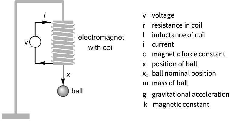
The affine model can be obtained directly from the governing equations:
assm = AffineStateSpaceModel[IconizedObject[«eqns»], {{x[t], Subscript[x, 0]}, {x'[t], 0}, {i[t], Subscript[x, 0]Sqrt[(m g/c)]}}, {{v[t], r Subscript[x, 0]Sqrt[(m g/c)]}}, x[t], t] /. IconizedObject[«pars»]The system without feedback is unstable, here with initial value {0.2,0.,0.1}:
OutputResponse[{assm, {0.2, 0, 0.1}}, 0, {t, 0, 5}];
Plot[%, {t, 0, 5}]
It is completely feedback linearizable, since it has no residual dynamics:
ℱ = FeedbackLinearize[assm, {{Subscript[z, 1], Subscript[z, 2], Subscript[z, 3]}, 𝒱}];ℱ["ResidualSystem"]The controller design based on the linear system:
κ1 = StateFeedbackGains[ℱ["LinearSystem"], {-1.5, -2 + I, -2 - I}]The closed-loop system using original state variables:
csys1 = ℱ[{"ClosedLoopSystem", κ1}];Simulate the system with initial value {0.3,0.,0.31305}:
OutputResponse[{csys1, {0.3, 0, 0.31305}}, 0, {t, 0, 6}];p1 = Plot[%, {t, 0, 6}]Design based on the approximately linearized system:
ssm = StateSpaceModel[assm];κ2 = StateFeedbackGains[ssm, {-1.5, -2 + I, -2 - I}]The closed-loop system with the controller based on linearization:
csys2 = SystemsModelStateFeedbackConnect[assm, κ2];Simulation of the system with controller based on approximate linearization:
OutputResponse[{csys2, {0.3, 0, 0.31305}}, 0, {t, 0, 35}];p2 = Plot[%, {t, 0, 35}, PlotStyle -> Dashed]The design based on feedback linearization has a better response:
OutputResponse[{csys2, {0.3, 0, 0.31305}}, 0, {t, 0, 35}];Show[Plot[%, {t, 0, 35}, PlotStyle -> Dashed], p1]Find a stabilizing controller for a two-wheeled inverted pendulum (e.g. Segway) using voltages to the two DC wheel motors as inputs:
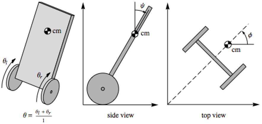
The AffineStateSpaceModel of the system with states {θ,θ',ψ,ψ',ϕ,ϕ'}:
asys = AffineStateSpaceModel[{{Subscript[θ, d],
   (4.905*Sin[ψ] - 245.25*Cos[ψ]*Sin[ψ] +
     (83.809 + 50.2854*Cos[ψ])*Subscript[θ, d] +
     Cos[ψ]*(-0.02499 + 1.25*Cos[ψ])*Sin[ψ]*
      Subscript[ϕ, d]^2 -
     83.8089*Subscript[ψ, d] - 50.2854*Cos[ψ]*
      Subscript[ψ, d] - 1.6866*Sin[ψ]*
      Subscript[ψ, d]^2)/(-1.7065 - 0.04*Cos[ψ] +
     Cos[ψ]^2), Subscript[ψ, d],
   (248.1923*Sin[ψ] + (-49.8831 - 50.2853*Cos[ψ])*
      Subscript[θ, d] - 1.265*Cos[ψ]*Sin[ψ]*
      Subscript[ϕ, d]^2 +
     49.883*Subscript[ψ, d] + 50.2853*Cos[ψ]*
      Subscript[ψ, d] - 0.02*Sin[ψ]*
      Subscript[ψ, d]^2 + Cos[ψ]*Sin[ψ]*
      Subscript[ψ, d]^2)/(-1.7065 - 0.04*Cos[ψ] +
     Cos[ψ]^2), Subscript[ϕ, d],
   (2*Subscript[ϕ, d]*(141.4276 + 2*Cos[ψ]*
       Sin[ψ]*Subscript[ψ, d]))/
    (-3.7992 + Cos[2*ψ])},
  {{0, 0}, {(-78.8557 - 47.3134*Cos[ψ])/(-1.7065 - 0.04*Cos[ψ] +
      Cos[ψ]^2), (-78.8557 - 47.3134*Cos[ψ])/
     (-1.7065 - 0.04*Cos[ψ] + Cos[ψ]^2)}, {0, 0},
   {(46.9349 + 47.3134*Cos[ψ])/(-1.7065 - 0.04*Cos[ψ] +
      Cos[ψ]^2), (46.9349 + 47.3134*Cos[ψ])/
     (-1.7065 - 0.04*Cos[ψ] + Cos[ψ]^2)}, {0, 0},
   {53.3193/(-3.7992 + Cos[2*ψ]), -53.3193/(-3.7992 + Cos[2*ψ])}},
  {θ, ϕ}, {{0, 0}, {0, 0}}},
 {θ, Subscript[θ, d], ψ,
  Subscript[ψ, d], ϕ,
  Subscript[ϕ, d]}, {Subscript[v, l],
  Subscript[v, r]}, {Automatic, Automatic}, Automatic,
 SamplingPeriod -> None];
Feedback linearize the system:
ℱ = FeedbackLinearize[asys]The zero dynamics have purely oscillatory behavior:
Eigenvalues@First@Normal@StateSpaceModel@ℱ["ZeroDynamicsSystem"];
Chop[%, 10^-4]
Design a controller using the linearized subsystem:
κ = StateFeedbackGains[ℱ["LinearSystem"]//N, {-4, -5, -6 + 3I , -6 - 3I}]Compute the state response of the closed-loop system:
csys = ℱ[{"ClosedLoopSystem", κ}];{θs, θsprime, ψs, ψsprime, ϕs, ϕsprime} = StateResponse[csys, (UnitStep[t] - UnitStep[t - 1]){2, 1}, {t, 0, 5}];The plots show that the oscillations are in the pendulum's pitch:
Table[Plot[res, {t, 0, 5}, PlotRange -> All], {res, {ψs, ψsprime}}]The two wheels are at rest in steady state:
Table[Plot[res, {t, 0, 5}, PlotRange -> All], {res, {θs, θsprime}}]And so is the yaw motion of the pendulum:
Table[Plot[res, {t, 0, 5}, PlotRange -> All], {res, {ϕs, ϕsprime}}]Mechanical Systems (2)
Design a vibration controller for a flexible structure, and compute the control effort expended. A two-mode model of a flexible structure with no damping: »
asys = AffineStateSpaceModel[{{Subscript[x, 2], 0, Subscript[x, 4],
   (-ω^2)*ArcTan[Subscript[x, 3]]}, {{0}, {1}, {0}, {1}},
  {Subscript[x, 1] - Subscript[x, 3]}, {{0}}},
 {Subscript[x, 1], Subscript[x, 2], Subscript[x, 3],
Subscript[x, 4]}, Automatic, {Automatic}, Automatic, SamplingPeriod -> None] /. ω -> 0.1;StateResponse[{asys, {1, 0, 1, 0}}, {0}, {t, 0, 200}];
Plot[#, {t, 0, 200}, PlotRange -> All]& /@ %[[{1, 3}]]The model is completely feedback linearizable:
ℱ = FeedbackLinearize[asys]Design a controller using the linear system to suppress the vibrations:
κ = StateFeedbackGains[ℱ["LinearSystem"], {-0.25, -0.75, -1 + 2I, -1 - 2I}]The modes of the closed-loop system:
sr = StateResponse[{ℱ[{"ClosedLoopSystem", κ}], {1, 0, 1, 0}}, {0}, {t, 0, 6}];Plot[#, {t, 0, 6}, PlotRange -> All]& /@ %[[{1, 3}]]OutputResponse[ℱ[{"OriginalSystemFullController", κ}], Join[{0}, sr], {t, 0, 6}];Plot[%, {t, 0, 6}, PlotRange -> All]Design a controller to suppress the oscillations in an axial flow compressor. A model of the compressor with throttle as input: »
asys = AffineStateSpaceModel[
 {{1.56 - ΔP + 1.5*(-1 + Subscript[m, c]) -
    0.5*(-1 + Subscript[m, c])^3,
   Subscript[m, c]/b},
  {{0}, {(-b^(-1))*ΔP}}, {Subscript[m, c]},
  {{0}}}, {{Subscript[m, c], 2.5413}, {ΔP, 2.0413}},
 {{Subscript[u, 1], 1.244938}}, {Automatic}, Automatic, SamplingPeriod -> None];
Simulations show the presence of surge-like oscillations:
ParametricPlot[Evaluate@StateResponse[asys /. b -> 2, 0, {t, 0, 200}], {t, 50, 200}]Feedback linearize the system:
ℱ = FeedbackLinearize[asys]Design a controller to suppress the oscillations:
StateFeedbackGains[ℱ["LinearSystem"], {-2 + I, -2 - I}]csys = ℱ[{"ClosedLoopSystem", %}]//SimplifySimulations show that the oscillations have been suppressed:
StateResponse[{csys, RandomReal[{0, 1}, 2]} /. b -> 2, 0, {t, 0, 10}];
Plot[%, {t, 0, 3}, PlotRange -> All]
Chemical Systems (1)
Design a controller to improve an isothermal continuous stirred-tank reactor process: »
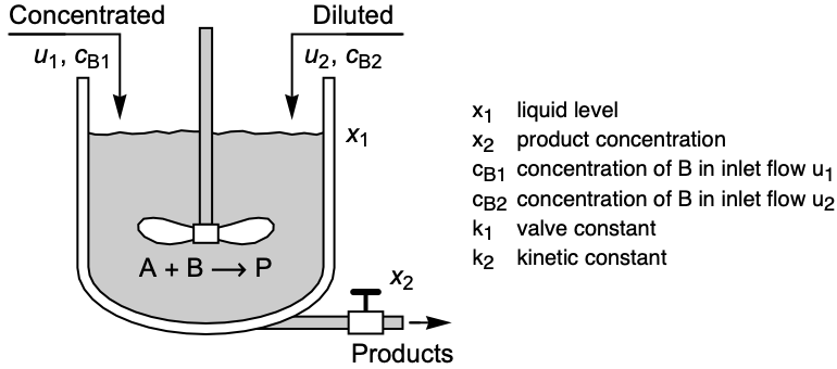
The affine system with states ![]() and inputs
and inputs ![]() :
:
pars = {Subscript[c, B1] -> 20.05, Subscript[c, B2] -> 0.2, Subscript[k, 1] -> 0.4, Subscript[k, 2] -> 1};asys = AffineStateSpaceModel[{{(-Subscript[k, 1])*Sqrt[Subscript[x, 1]],
((-Subscript[k, 2])*Subscript[x, 2])/
(1 + Subscript[x, 2])^2},
{{1, 1}, {(Subscript[c, B1] - Subscript[x, 2])/
Subscript[x, 1], (Subscript[c, B2] -
Subscript[x, 2])/Subscript[x, 1]}},
{Subscript[x, 1], Subscript[x, 2]}, {{0, 0}, {0, 0}}},
{{Subscript[x, 1], 25.05}, {Subscript[x, 2], 9}},
{{Subscript[u, 1], 1}, {Subscript[u, 2], 1}}, {Automatic, Automatic},
Automatic, SamplingPeriod -> None];The system is completely feedback linearizable:
ℱ = FeedbackLinearize[asys]Design a controller based on the linearized system:
κ = StateFeedbackGains[ℱ["LinearSystem"], {-2 + 2I, -2 - 2I}]csys = ℱ[{"ClosedLoopSystem", κ}]The response of the closed-loop system from a non-equilibrium initial condition:
StateResponse[AffineStateSpaceModel[csys /. pars, {Subscript[x, 1] -> 35, Subscript[x, 2] -> 2.5}], UnitStep[t]{1, 1}, {t, 0, 2}];
p = Plot[%, {t, 0, 2}, PlotRange -> All]
The response of the uncontrolled system is far worse:
StateResponse[AffineStateSpaceModel[asys /. pars, {Subscript[x, 1] -> 35, Subscript[x, 2] -> 2.5}], UnitStep[t]{1, 1}, {t, 0, 2}];Show[p, Plot[%, {t, 0, 2}, PlotRange -> All, PlotStyle -> Dashed]]Assume that the inputs to the system are random and normally distributed:
rInp := Interpolation@Thread[{Range[0, 5, 0.5], RandomVariate[NormalDistribution[1, 1], 11]}]The response of the controlled system:
Table[StateResponse[AffineStateSpaceModel[csys /. pars, {Subscript[x, 1] -> 26, Subscript[x, 2] -> 8}], rInp[t]{1, 1}, {t, 0, 5}], {3}];
p1 = Plot[Evaluate[%], {t, 0, 5}]
The response of the open-loop system:
Table[StateResponse[AffineStateSpaceModel[asys /. pars, {Subscript[x, 1] -> 26, Subscript[x, 2] -> 8}], rInp[t]{1, 1}, {t, 0, 5}], {3}];
p2 = Plot[Evaluate[%], {t, 0, 5}, PlotStyle -> Dashed]
Again, the response of the controlled system is better:
Show[p2, p1, Plot[{25, 9}, {t, 0, 5}, IconizedObject[«plotOpts»]]]Electrical Systems (2)
Design a controller for better speed response in an induction motor subject to varying loads: »
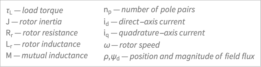
The model of the motor with inputs ![]() :
:
pars = {Subscript[n, p] -> 1, J -> 0.09, M -> 0.07, Subscript[L, r] -> 0.07, Subscript[R, r] -> 0.3};imotor = AffineStateSpaceModel[{{(-J^(-1))*Subscript[τ, L],
(-Subscript[L, r]^(-1))*Subscript[R, r]*
Subscript[ψ, d], ω*
Subscript[n, p]},
{{((-J^(-1))*M*Subscript[n, p]*
Subscript[ψ, d])/Subscript[L, r], 0},
{0, (M*Subscript[R, r])/
Subscript[L, r]},
{(M*(Subscript[R, r]/Subscript[ψ,
d]))/Subscript[L, r], 0}},
{ω, ρ}, {{0, 0}, {0, 0}}},
{{ω, 100}, {Subscript[ψ, d], -0.2739},
{ρ, 0.2}}, {{Subscript[i, q], 91.2871},
{Subscript[i, d], -3.9123}}, {Automatic, Automatic}, Automatic,
SamplingPeriod -> None] /. pars;Simulations show the effect of torque on the angular velocity:
Table[Tooltip[StateResponse[{imotor, {100, -0.2, 0.1}}, {91.2871, -3.9123}, {t, 0, 6}][[1]], Subscript[τ, L]], {Subscript[τ, L], {0, 10, 15, 20, 25, 30, 35, 36}}];Plot[Evaluate[%], {t, 0, 6}, PlotRange -> {All, {0, 300}}, PlotStyle -> Dashed]The model with an integrator in the q axis:
imotorq = SystemsModelSeriesConnect[StateSpaceModel[{{{0}}, {{1, 0}}, {{1}, {0}}, {{0, 0}, {0, 1}}}, {{Subscript[i, q], 91.2871}},
 {{Subscript[v, 1], 0}, {Subscript[v, 2], -3.9123}}, SamplingPeriod -> None,
 SystemsModelLabels -> None], imotor]
Feedback linearize the system:
ℱ = FeedbackLinearize[imotorq]Design a state feedback controller for the linear system:
κ = StateFeedbackGains[ℱ["LinearSystem"]//N, {-3 - I , -3 + I, -4, -5}]csys = ℱ[{"ClosedLoopSystem", κ}]//Simplify//ChopSimulate the closed-loop system for various torque values:
Table[Tooltip[StateResponse[{csys, {91 , 80, -0.2, 0.1}}, {0, 0}, {t, 0, 3}][[2]], Subscript[τ, L]], {Subscript[τ, L], {0, 10, 15, 20, 25, 30, 35, 36}}];Plot[Evaluate[%], {t, 0, 3}, PlotRange -> All]Design a controller that regulates quantities in a wind energy conversion system: »
asys = AffineStateSpaceModel[{{-0.21798365122615806*Subscript[i, md] +
    37.19969202258031*Subscript[v, DC] +
    Subscript[i, mq]*(-13.623978201634879 -
      0.6811989100817439*Subscript[ω, m]) -
    204.35967302452318*Subscript[ω, m],
   -0.32*Subscript[i, mq] + 362.13068117068144*
     Subscript[v, DC] - 1805.8534058534062*
     Subscript[ω, m] + Subscript[i, md]*
     (29.36 + 1.4679999999999997*Subscript[ω, m]),
   -5.606732673267327*^-6*(-259.0002590002591 + 1.*Subscript[i, md])*
     (300. + Subscript[i, mq]) -
    8.712871287128714/(20. + Subscript[ω, m]),
   -5.960464477539063*^-8 - 136522.86972286974*Subscript[i, md] -
    905326.7029267036*Subscript[i, mq] -
    21569.290876560284*Subscript[i, nd] -
    2.7408892835212727*^6*Subscript[i, nq],
   -2.9152542372881354*Subscript[i, nd] -
    1.*Ω*Subscript[i, nq] +
    73.11624025952639*Subscript[v, DC],
   1.*Ω*Subscript[i, nd] -
    2.9152542372881354*Subscript[i, nq] +
    9291.150113631433*Subscript[v, DC]},
  {{272.47956403269757 + 2.7247956403269757*Subscript[v, DC], 0, 0, 0},
   {0, 400. + 4.*Subscript[v, DC], 0, 0}, {0, 0, 0, 0},
   {-10000.*(-1684.641284641285 + Subscript[i, md]),
    -10000*(300 + Subscript[i, mq]),
    -10000.*(-46404.73361900462 + Subscript[i, nd]),
    -10000*(350 + Subscript[i, nq])},
   {0, 0, 3389.8305084745766 + 33.898305084745765*Subscript[v, DC], 0},
   {0, 0, 0, 3389.8305084745766 + 33.898305084745765*Subscript[v, DC]}},
  {Subscript[ω, m], Subscript[i, md],
   Subscript[i, nq], Subscript[v, DC]},
  {{0, 0, 0, 0}, {0, 0, 0, 0}, {0, 0, 0, 0}, {0, 0, 0, 0}}},
 {Subscript[i, md], Subscript[i, mq],
  Subscript[ω, m], Subscript[v, DC],
  Subscript[i, nd], Subscript[i, nq]},
 {Subscript[U, md], Subscript[U, mq],
  Subscript[U, nd], Subscript[U, nq]},
{Automatic, Automatic, Automatic, Automatic}, Automatic, SamplingPeriod -> None];ℱ = FeedbackLinearize[asys]StateSpaceModel@ℱ["ZeroDynamicsSystem"];
Eigenvalues@First@Normal[%] /. Ω -> 0The linear system consists of a double integrator and three single integrators:
lsys = TransferFunctionModel@ℱ["LinearSystem"]A controller that gives desired closed-loop transfer functions in each linearized and decoupled loop:
ctr = TransferFunctionModel[Unevaluated[{{((12 + 16.55 s)/7.2 + s), 0, 0, 0}, {0, 4, 0, 0}, {0, 0, 5, 0}, {0, 0, 0, 6}}], s, SamplingPeriod -> None, SystemsModelLabels -> None];csysl = SystemsModelFeedbackConnect[lsys, ctr]//TransferFunctionCancelThe closed-loop system also has the same linear characteristics plus the zero dynamics:
csys = ℱ[{"ClosedLoopSystem", ctr}];
Eigenvalues@First@Normal@StateSpaceModel[csys] /. Ω -> 0
The response of the system to a unit step applied to each input in turn:
y = OutputResponse[{csys /. Ω -> 0}, UnitStep[t], {t, 0, 5}];The first input affects only the first output:
Plot[y[[1]], {t, 0, 5}]And the closed-loop behaves as the designed linear system:
yl = OutputResponse[csysl, UnitStep[t], {t, 0, 5}];
Plot[yl[[1]], {t, 0, 5}]
This is true of the three other decoupled SISO loops as well:
Table[{Plot[y[[i]], {t, 0, 5}], Plot[yl[[i]], {t, 0, 5}]}, {i, {2, 3, 4}}]Properties & Relations (9)
The linear system lsys is given in Burnovsky form:
asys = AffineStateSpaceModel[{{Subscript[x, 2] + Subscript[x, 2]^2,
Subscript[x, 3] - Subscript[x, 1]*Subscript[x, 4] +
Subscript[x, 4]*Subscript[x, 5],
-Subscript[x, 2]^2 + Subscript[x, 2]*Subscript[x, 4] +
Subscript[x, 1]*Subscript[x, 5], Subscript[x, 5],
Subscript[x, 2]^2}, {{0, 1}, {0, 0},
{Cos[Subscript[x, 1] - Subscript[x, 5]], 1}, {0, 0}, {0, 1}},
{Subscript[x, 1] - Subscript[x, 5], Subscript[x, 4]},
{{0, 0}, {0, 0}}}, {Subscript[x, 1], Subscript[x, 2],
Subscript[x, 3], Subscript[x, 4], Subscript[x, 5]},
{Subscript[, 1], Subscript[, 2]}, {Automatic, Automatic}, Automatic, SamplingPeriod -> None];The Burnovsky form consists of chains of integrators:
lsys = FeedbackLinearize[asys, Automatic, "LinearSystem"];{lsys, TransferFunctionModel[lsys]}The length of integrator chains is determined by the relative orders:
SystemsModelVectorRelativeOrders[asys]The Burnovsky form is controllable and observable:
lsys = FeedbackLinearize[AffineStateSpaceModel[{{4*Subscript[x, 1]^3 + Subscript[x, 2],
Subscript[x, 3], 0}, {{0}, {0}, {1}}, {Subscript[x, 1]}, {{0}}},
{Subscript[x, 1], Subscript[x, 2], Subscript[x, 3]},
{Subscript[, 1]}, {Automatic}, Automatic, SamplingPeriod -> None], Automatic, "LinearSystem"]{ControllableModelQ[lsys], ObservableModelQ[lsys]}The order of the linear system is the sum of the relative orders:
asys = AffineStateSpaceModel[{{Subscript[x, 1]*Subscript[x, 2],
   -Subscript[x, 2], Subscript[x, 1]*Subscript[x, 4],
   Subscript[x, 2]}, {{Subscript[x, 1], 1},
   {1 + Subscript[x, 3], 0}, {0, 1}, {Subscript[x, 2],
    -1 + Subscript[x, 1]}}, {Subscript[x, 1],
   Subscript[x, 3]}, {{0, 0}, {0, 0}}}, {Subscript[x, 1],
  Subscript[x, 2], Subscript[x, 3], Subscript[x, 4]},
 {Subscript[u, 1], Subscript[u, 2]}, {Automatic, Automatic}, Automatic,
SamplingPeriod -> None];ℱ = FeedbackLinearize[asys];{SystemsModelOrder[ℱ["LinearSystem"]], Total@SystemsModelVectorRelativeOrders[asys]}Since the order of the linear system lsys is less than 4, there are residual dynamics:
ℱ["ResidualSystem"]The modes of the zero dynamics of a linear system are its transmission zeros:
tfm = TransferFunctionModel[
 {{{(s + Subscript[z, 1])*(s +
      Subscript[z, 2])}}, s^4 + Subscript[a, 0] +
   s*Subscript[a, 1] + s^2*Subscript[a, 2] +
   s^3*Subscript[a, 3]}, s, SamplingPeriod -> None,
SystemsModelLabels -> None];zdynamics = FeedbackLinearize[AffineStateSpaceModel[tfm], Automatic, "ZeroDynamicsSystem", Method -> "Burnovsky"];Eigenvalues@First@Normal@StateSpaceModel@zdynamicsThe problem of zeroing the output:
asys = AffineStateSpaceModel[{{Cos[Subscript[x, 1]], Subscript[x, 1]*
    Subscript[x, 2], -Subscript[x, 2], Subscript[x, 3]},
  {{1 + Subscript[x, 4], 0}, {0, 1 + Subscript[x, 1]}, {0, 0},
   {Subscript[x, 2], Subscript[x, 3]}},
  {Subscript[x, 1], Subscript[x, 2]}, {{0, 0}, {0, 0}}},
 {Subscript[x, 1], Subscript[x, 2], Subscript[x, 3],
  Subscript[x, 4]}, {Subscript[u, 1], Subscript[u, 2]},
{Automatic, Automatic}, Automatic, SamplingPeriod -> None];ℱ = FeedbackLinearize[asys, {{Subscript[z, 1], Subscript[z, 2], Subscript[z, 3], Subscript[z, 4]}, {Subscript[v, 1], Subscript[v, 2]}}];The trajectories of the zero dynamics:
zdresp = OutputResponse[{ℱ["ZeroDynamicsSystem"], {1, 1}}, {}, {t, 0, 200}]The inverse state transformation:
xtrans = First@Solve[Equal@@@ℱ["InverseStateTransformation"], {Subscript[x, 1], Subscript[x, 2], Subscript[x, 3], Subscript[x, 4]}]Compute the input that gives zero output:
Last /@ ℱ["InverseFeedbackTransformation"] /. xtrans /. Thread[{Subscript[z, 1], Subscript[z, 2], Subscript[z, 3], Subscript[z, 4]} -> Join[{0, 0}, zdresp]];inp = {Subscript[u, 1], Subscript[u, 2]} /. Solve[% == 0, {Subscript[u, 1], Subscript[u, 2]}]//FlattenThe output is essentially zero for the nonzero input:
OutputResponse[{asys, {0, 0, 1, 1}}, inp, {t, 0, 200}];
{Plot[inp, {t, 0, 200}, PlotRange -> All], Plot[Chop[%], {t, 0, 200}, PlotRange -> All]}
The linear system lsys together with the residual system rsys gives the transformed system:
asys = AffineStateSpaceModel[{{Cos[Subscript[x, 1]], Subscript[x, 1]*
    Subscript[x, 2], -Subscript[x, 2], Subscript[x, 3]},
  {{1 + Subscript[x, 4], 0}, {0, 1 + Subscript[x, 1]}, {0, 0},
   {Subscript[x, 2], Subscript[x, 3]}},
  {Subscript[x, 1], Subscript[x, 2]}, {{0, 0}, {0, 0}}},
 {Subscript[x, 1], Subscript[x, 2], Subscript[x, 3],
  Subscript[x, 4]}, {Subscript[u, 1], Subscript[u, 2]},
{Automatic, Automatic}, Automatic, SamplingPeriod -> None];ℱ = FeedbackLinearize[asys, {{Subscript[z, 1], Subscript[z, 2], Subscript[z, 3], Subscript[z, 4]}, {Subscript[v, 1], Subscript[v, 2]}}];The transformed system tsys has lsys and rsys in parallel:
tsys = SystemsModelMerge[{ℱ["LinearSystem"], SystemsModelDelete[ℱ["ResidualSystem"], None, All]}]Obtain it directly from the linearization data object:
ℱ["TransformedSystem"]Obtain the transformed system from the original system using feedback and coordinate transformation:
asys = AffineStateSpaceModel[{{Cos[Subscript[x, 1]], Subscript[x, 1]*
    Subscript[x, 2], -Subscript[x, 2], Subscript[x, 3]},
  {{1 + Subscript[x, 4], 0}, {0, 1 + Subscript[x, 1]}, {0, 0},
   {Subscript[x, 2], Subscript[x, 3]}},
  {Subscript[x, 1], Subscript[x, 2]}, {{0, 0}, {0, 0}}},
 {Subscript[x, 1], Subscript[x, 2], Subscript[x, 3],
  Subscript[x, 4]}, {Subscript[u, 1], Subscript[u, 2]},
{Automatic, Automatic}, Automatic, SamplingPeriod -> None];ℱ = FeedbackLinearize[asys, {{Subscript[z, 1], Subscript[z, 2], Subscript[z, 3], Subscript[z, 4]}, {Subscript[v, 1], Subscript[v, 2]}}];fb = ℱ["FeedbackCompensator"];SystemsModelSeriesConnect[fb, asys];
StateSpaceTransform[%, {{Subscript[x, 1], Subscript[x, 2], Subscript[x, 3], Subscript[x, 4]}, ℱ["InverseStateTransformation"]}]It can also be obtained by first applying the transformation and then feedback:
fb /. First[Solve[Equal@@@ℱ["InverseStateTransformation"], {Subscript[x, 1], Subscript[x, 2], Subscript[x, 3], Subscript[x, 4]}]];StateSpaceTransform[asys, {{Subscript[x, 1], Subscript[x, 2], Subscript[x, 3], Subscript[x, 4]}, ℱ["InverseStateTransformation"]}];SystemsModelSeriesConnect[%%, %]The original system can be reacquired from the transformed system:
asys = AffineStateSpaceModel[{{Cos[Subscript[x, 1]], Subscript[x, 1]*
    Subscript[x, 2], -Subscript[x, 2], Subscript[x, 3]},
  {{1 + Subscript[x, 4], 0}, {0, 1 + Subscript[x, 1]}, {0, 0},
   {Subscript[x, 2], Subscript[x, 3]}},
  {Subscript[x, 1], Subscript[x, 2]}, {{0, 0}, {0, 0}}},
 {Subscript[x, 1], Subscript[x, 2], Subscript[x, 3],
  Subscript[x, 4]}, {Subscript[u, 1], Subscript[u, 2]},
{Automatic, Automatic}, Automatic, SamplingPeriod -> None];ℱ = FeedbackLinearize[asys, {{Subscript[z, 1], Subscript[z, 2], Subscript[z, 3], Subscript[z, 4]}, {Subscript[v, 1], Subscript[v, 2]}}];tsys = ℱ["TransformedSystem"];The feedback transformation ![]() as a static system:
as a static system:
ifb = ℱ["InverseFeedbackCompensator"]Apply the feedback followed by the state transform to tsys:
ztrans = ℱ["InverseStateTransformation"];StateSpaceTransform[SystemsModelSeriesConnect[ifb, tsys], {ztrans, {Subscript[x, 1], Subscript[x, 2], Subscript[x, 3], Subscript[x, 4]}}]Apply the state transform followed by the feedback to tsys:
SystemsModelSeriesConnect[ifb, StateSpaceTransform[tsys, {ztrans, {Subscript[x, 1], Subscript[x, 2], Subscript[x, 3], Subscript[x, 4]}}]]NonlinearStateSpaceModel[asys]The zero dynamics are obtained from the residual dynamics by deleting all the inputs:
asys = AffineStateSpaceModel[{{Cos[Subscript[x, 1]], Subscript[x, 1]*
    Subscript[x, 2], -Subscript[x, 2], Subscript[x, 3]},
  {{1 + Subscript[x, 4], 0}, {0, 1 + Subscript[x, 1]}, {0, 0},
   {Subscript[x, 2], Subscript[x, 3]}},
  {Subscript[x, 1], Subscript[x, 2]}, {{0, 0}, {0, 0}}},
 {Subscript[x, 1], Subscript[x, 2], Subscript[x, 3],
  Subscript[x, 4]}, {Subscript[u, 1], Subscript[u, 2]},
{Automatic, Automatic}, Automatic, SamplingPeriod -> None];ℱ = FeedbackLinearize[asys, {{Subscript[z, 1], Subscript[z, 2], Subscript[z, 3], Subscript[z, 4]}, {Subscript[v, 1], Subscript[v, 2]}}];{ℱ["ZeroDynamics"], SystemsModelDelete[ℱ["ResidualSystem"], All]}Possible Issues (1)
A nonidentity feedback causes a mismatch between the specified and actual estimator poles:
asys = AffineStateSpaceModel[{{Subscript[x, 2],
   -5.880000000000002*Sin[Subscript[x, 1]] - 100*Subscript[x, 1] -
    Subscript[x, 2] + 100*Subscript[x, 3] + Subscript[x, 4],
   Subscript[x, 4], 2.5*(100*Subscript[x, 1] +
     Subscript[x, 2] - 100*Subscript[x, 3] -
     Subscript[x, 4])}, {{0}, {0}, {0}, {2.5}}, {Subscript[x, 1]},
  {{0}}}, {Subscript[x, 1], Subscript[x, 2],
  Subscript[x, 3], Subscript[x, 4]}, Automatic, {Automatic}, Automatic,
SamplingPeriod -> None];ℱ = FeedbackLinearize[asys];ℱ["InverseFeedbackTransformation"]This may cause the estimator to be unstable:
ℱ[{"OriginalSystemEstimator", EstimatorGains[ℱ["LinearSystem"], {-1, -2, -3}]}];Eigenvalues@First@Normal@StateSpaceModel[%]Adjust the pole specifications to obtain a stable estimator:
ℱ[{"OriginalSystemEstimator", EstimatorGains[ℱ["LinearSystem"], 70{-1, -2, -3}]}];Eigenvalues@First@Normal@StateSpaceModel[%]Text
Wolfram Research (2014), FeedbackLinearize, Wolfram Language function, https://reference.wolfram.com/language/ref/FeedbackLinearize.html.
CMS
Wolfram Language. 2014. "FeedbackLinearize." Wolfram Language & System Documentation Center. Wolfram Research. https://reference.wolfram.com/language/ref/FeedbackLinearize.html.
APA
Wolfram Language. (2014). FeedbackLinearize. Wolfram Language & System Documentation Center. Retrieved from https://reference.wolfram.com/language/ref/FeedbackLinearize.html