

DiscreteHilbertTransform
DiscreteHilbertTransform[list]
finds the discrete Hilbert transform of the list list of real numbers.
Details
- Discrete Hilbert transforms have applications in signal processing, communications, acoustics, data compression, seismic ambient data, gravitational waves, etc.
- This transform imparts a
 phase shift to the original sequence for positive frequencies and a
  phase shift for negative frequencies.
 - For a list
 , DiscreteHilbertTransform, calculates its FFT, annihilates negative frequencies and calculates the inverse FFT of the result, of which the imaginary part is
  . »
. » - In signal processing, the complex sequence
 is called the analytic signal, and its magnitude is the envelope:
  can have any positive integer length.
 - If the elements of
 are exact numbers, DiscreteHilbertTransform begins by applying N to them.
  can also be a SparseArray object, resulting in
  , also a SparseArray object.
Examples
open all close allBasic Examples (2)
Scope (9)
x = {1, 0, 0, 1, 0, 0, 1};Compute the discrete Hilbert transform with machine arithmetic:
DiscreteHilbertTransform[x]Compute using 24-digit precision arithmetic:
DiscreteHilbertTransform[N[x, 24]]Compute a 2D discrete Hilbert transform:
DiscreteHilbertTransform[RandomReal[{2, 4}, {3, 6}]]x is a rank-3 tensor with nonzero diagonal:
x = ConstantArray[0, {2, 3, 4}];x[[1, 1, 1]] = 1;x[[2, 2, 2]] = 1;Compute the 3D Discrete Hilbert transform:
DiscreteHilbertTransform[x]x is a SparseArray of real values:
x = SparseArray[{{1, 2} -> -1, {2, 2} -> 2π, {3, 3} -> 1.3, {2, 3} -> 7}];Compute the discrete Hilbert transform and get the result as a SparseArray:
DiscreteHilbertTransform[x]x is a large sparse matrix of real values:
x = SparseArray[Table[3 ^ i -> 1, {i, 10}]];Compute the discrete Hilbert transform and get the result as a SparseArray:
DiscreteHilbertTransform[x]Consider a discrete cosine wave:
discreteCosine = Table[Cos[t], {t, -π, π, π / 25}];DiscreteHilbertTransform applies a ![]() degree phase shift:
degree phase shift:
discreteHCosine = DiscreteHilbertTransform[discreteCosine];ListPlot[{discreteCosine, discreteHCosine}, ...]Here are the values for the first 10 elements of the discrete signal and its discrete Hilbert transform:
Tabular[(Transpose[{N[discreteCosine], discreteHCosine}])[[ ;; 10]] , {...}]Generate a random sequence of real numbers:
x = RandomReal[1, 200];Compute the discrete Hilbert transform:
dhtx = DiscreteHilbertTransform[x];Plot the original data and its transform together:
ListLinePlot[{x, dhtx}, ...]Consider instead a sinusoidal sequence with some noise:
x = Sin[17 * 2π * Range[0, 1, 0.001]] + RandomVariate[NormalDistribution[0, 0.05], 1001];Compute the discrete Hilbert transform:
dhtx = DiscreteHilbertTransform[x];Plot the original data and its transform together:
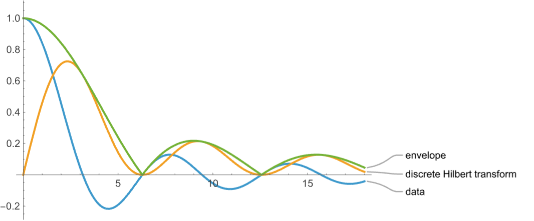
ListLinePlot[{x, dhtx}, ...]Data from a Sinc function with noise:
n = 100;
x = Table[Sinc[x - 10], {x, n}] + RandomReal[{-.05, .05}, {n}];ListPlot[x, PlotRange -> All]p = Fourier[x, FourierParameters -> {1, 1}];
ListPlot[Abs[p] ^ 2]Its discrete Hilbert transform:
dHx = DiscreteHilbertTransform[x];It provides the imaginary component for the analytic representation:
a = x + I * dHx;Power spectrum for the analytical signal:
s = Fourier[a, FourierParameters -> {1, 1}];
ListPlot[Abs[s] ^ 2]
The envelope of an oscillating signal is a curve outlining its extremes, and it is the magnitude of the
analytic representation:
ListLinePlot[{x, dHx, Abs /@ a}, ...]Applications (4)
Communications (1)
Consider the following message signal:
m = Table[Sin[2Pi 5t] + 2Sin[2Pi 7t] + 1 / 2Sin[2Pi 9t], {t, -π / 2, π / 2, π / 100}];
ListLinePlot[m, DataRange -> {-π / 2, π / 2}, ...]
Using ![]() as a message carrier, get the upper side band-suppressed carrier (USB-SC) and lower side band-suppressed carrier (LSB-SC):
as a message carrier, get the upper side band-suppressed carrier (USB-SC) and lower side band-suppressed carrier (LSB-SC):
c = Table[Cos[2Pi 55t], {t, -π / 2, π / 2, π / 100}];
s = Table[Sin[2Pi 55t], {t, -π / 2, π / 2, π / 100}];
USB = m * c - DiscreteHilbertTransform[m] * s;
LSB = m * c + DiscreteHilbertTransform[m] * s;
ListLinePlot[{USB, LSB}, ...]
ECG Frequency Analysis (1)
Electrocardiogram time-frequency analysis can reveal important information. Consider a patient's ECG data, which provides a voltage versus time graph of the electrical activity of the heart:
ECGData = {...};
ListLinePlot[ECGData, ...]
Filter the data using KaiserWindow:
filteredECG = BandpassFilter[ECGData, {(4π/25), (2π/5)}, Length[ECGData], KaiserWindow];Find its first differential in the discrete domain(sampling frequency of 100Hz):
differentialECG = Differences[filteredECG] / (2 * .01);The discrete Hilbert transform is:
dhDifferentialECG = DiscreteHilbertTransform[differentialECG];Compare the RMS and 18% of the maximum of the discrete Hilbert transform:
{Max[dhDifferentialECG] * .18, RootMeanSquare[dhDifferentialECG]}This will indicate a threshold of 39% of the maximum: with this information, you can now find the location of the R peaks using the Hilbert transform of the first differential:
RpeaksLocation = First /@ FindPeaks[dhDifferentialECG, Automatic, Automatic, Max[dhDifferentialECG] * .39];Visualize R peaks in the ECG data:
RPeaks = Transpose@{RpeaksLocation, ECGData[[RpeaksLocation]]};
ListPlot[{ECGData, RPeaks}, ...]
Wind Speed Prediction (1)
Consider the weather forecast for wind speed and direction in the city of San Juan, Puerto Rico, for the next seven days:
speedDateData = QuantityMagnitude[WeatherForecastData[...]];
directionDateData = (π/180)QuantityMagnitude[WeatherForecastData[...]];
DateListPlot[{speedDateData, directionDateData}, ...]
The predicted wind speed is given by the formula ![]() , where
, where ![]() is the maximum value of the speed data and
is the maximum value of the speed data and ![]() and
and ![]() are the mean values for the sequences
are the mean values for the sequences ![]() and direction data, respectively.
and direction data, respectively. ![]() and
and ![]() are the discrete Hilbert transforms for these sequences, respectively, with their mean values removed:
are the discrete Hilbert transforms for these sequences, respectively, with their mean values removed:
{...};
DateListPlot[{...}, ...]
Seismic Data Analysis (1)
Consider the following seismic trace, which illustrates how ground motion, resulting from seismic waves, is detected and recorded over time:
trace = {...};
ListLinePlot[trace]
Compute its Hilbert transform:
dhTrace = DiscreteHilbertTransform[trace];complexTrace = trace + I * dhTrace;env = Abs[complexTrace];Plot the trace, its transform and its envelope:
ListLinePlot[{trace, dhTrace, env, -env}, ...]phase = ArcTan[trace, dhTrace];
ListLinePlot[phase, PlotLabel -> "Instantaneous phase for the complex trace"]Properties & Relations (2)
Subscript[f, k] = {1.1, -1.2, 5.5, -4.5};Calculate its fast Fourier transform:
fFourier = Fourier[Subscript[f, k], FourierParameters -> {1, -1}]Annihilate negative frequencies:
anhilation = {1, 2, 1, 0} * fFourierInverseFourier[anhilation, FourierParameters -> {1, -1}]Finally, compare the imaginary part with DiscreteHilbertTransform:
Im[%] == DiscreteHilbertTransform[Subscript[f, k]]For the analytic representation of a real value signal:
{-2.3, -3.14, 1.62, E, Pi} + I DiscreteHilbertTransform[{-2.3, -3.14, 1.62, E, Pi}]The DC component (first position) and the Nyquist component(![]() position) are always real:
position) are always real:
Fourier[%, FourierParameters -> {1, -1}]//ChopText
Wolfram Research (2026), DiscreteHilbertTransform, Wolfram Language function, https://reference.wolfram.com/language/ref/DiscreteHilbertTransform.html.
CMS
Wolfram Language. 2026. "DiscreteHilbertTransform." Wolfram Language & System Documentation Center. Wolfram Research. https://reference.wolfram.com/language/ref/DiscreteHilbertTransform.html.
APA
Wolfram Language. (2026). DiscreteHilbertTransform. Wolfram Language & System Documentation Center. Retrieved from https://reference.wolfram.com/language/ref/DiscreteHilbertTransform.html