Wolfram Language & System Documentation Center

HilbertTransform

HilbertTransform[f[t],t,s]

gives the symbolic Hilbert transform of f[t] in the variable t and returns a transform F[s] in the variable s.

HilbertTransform[f[t],t,]

gives the numeric Hilbert transform at the numerical value .

Details and Options

Hilbert transforms are used to solve problems in signal processing, communications and other fields.
The Hilbert transform of a function is defined to be principal value integral .
HilbertTransform shifts every frequency component of a function by a phase of radians.
The conjugate function is the analytic representation of , and its magnitude is the envelope:

HilbertTransform is a singular integral transform. Moreover, it is a bounded operator on $L^p(TemplateBox[{}, Reals])$ for .
The integral is computed using numerical methods if the third argument, , is given a numerical value.
The following options can be given:

AccuracyGoal	Automatic	digits of absolute accuracy sought
Assumptions	$Assumptions	assumptions to make about parameters
GenerateConditions	Automatic	whether to generate answers that involve conditions on parameters
Method	Automatic	method to use
PrecisionGoal	Automatic	digits of precision sought
WorkingPrecision	Automatic	the precision used in internal computations

Examples

open all close all

Basic Examples (4)

Compute the Hilbert transform of a function:

Wolfram Language code: HilbertTransform[Sin[t], t, s]

Plot the function and its Hilbert transform:

Wolfram Language code: {Plot[Sin[t], {t, -2Pi, 2Pi}], Plot[%, {s, -2Pi, 2Pi}]}

Hilbert transform of :

Wolfram Language code: HilbertTransform[DiracDelta[t], t, s]

Hilbert transform of a Cauchy pulse:

Wolfram Language code: HilbertTransform[1 / (1 ^ 2 + t ^ 2), t, s]

Plot both:

Wolfram Language code: {Plot[1 / (1 ^ 2 + t ^ 2), {t, -5, 5}], Plot[%, {s, -5, 5}]}

Compute the transform at a single point:

Wolfram Language code: HilbertTransform[Cos[t] - Sin[t], t, 1.3]

Scope (29)

Basic Uses (4)

Hilbert transform of a function for a symbolic parameter :

Wolfram Language code: HilbertTransform[Exp[2 I t], t, s]

Hilbert transforms of simple trigonometric functions:

Wolfram Language code: HilbertTransform[Sin[α t], t, s, Assumptions -> α > 0]

Wolfram Language code: HilbertTransform[Cos[α t], t, s, Assumptions -> α < 0]

Evaluate the Hilbert transform for a numerical value of the parameter :

Wolfram Language code: HilbertTransform[UnitBox[t], t, 0.3]

TraditionalForm formatting:

Wolfram Language code: HilbertTransform[f[t], t, s]//TraditionalForm

Elementary Functions (5)

Parabolic pulse:

Wolfram Language code: HilbertTransform[Piecewise[{{1 - t ^ 2, Abs[t] <= 1}, {0, Abs[t] > 1}}], t, t]

Plot both:

Wolfram Language code: Plot[{Piecewise[{{1 - t ^ 2, Abs[t] <= 1}, {0, Abs[t] > 1}}], %}, ...]

Square pulse:

Wolfram Language code: HilbertTransform[UnitBox[t], t, t]

Plot both:

Wolfram Language code: Plot[{UnitBox[t], %}, {t, -2, 2}, ...]

Bipolar pulse:

Wolfram Language code: HilbertTransform[UnitBox[t]Sign[t], t, t]

Plot both:

Wolfram Language code: Plot[{UnitBox[t]Sign[t], %}, {t, -2, 2}, ...]

Double triangle pulse:

Wolfram Language code: HilbertTransform[t UnitBox[t]Sign[t], t, t]

Plot both:

Wolfram Language code: Plot[{t UnitBox[t]Sign[t], %}, {t, -2, 2}, ...]

One-sided rectangular pulse:

Wolfram Language code: HilbertTransform[UnitBox[t - 1 / 2], t, t]

Wolfram Language code: Plot[{UnitBox[t - 1 / 2], %}, {t, -5, 5}, ...]

Trigonometric Functions (4)

Quotient of trigonometric and linear functions:

Wolfram Language code: HilbertTransform[Sin[3 t] / t, t, t]

Plot both:

Wolfram Language code: Plot[{Sin[3 t] / t, %}, {t, -2, 2}]

Wolfram Language code: HilbertTransform[Cos[-4 t] / t, t, t]

Plot both:

Wolfram Language code: Plot[{Cos[-4 t] / t, %}, {t, -2, 2}]

Quotient of trigonometric and monomial functions:

Wolfram Language code: HilbertTransform[Sin[a t] / t ^ 2, t, s, Assumptions -> a > 0]

Products of cosine functions:

Wolfram Language code: HilbertTransform[Cos[a t] ^ 3, t, s, Assumptions -> a > 0]

Wolfram Language code: HilbertTransform[Cos[a t] ^ 5, t, s, Assumptions -> a > 0]

Wolfram Language code: HilbertTransform[Cos[α t + ϕ] Cos[β t + Φ], t, s, Assumptions -> 0 < α < β]

Composition of elementary functions:

Wolfram Language code: HilbertTransform[Sin[t ^ 2], t, t]

Plot both:

Wolfram Language code: Plot[{Sin[t ^ 2], %}, {t, -5, 5}]

Powers and Algebraic Functions (5)

Rational functions with linear denominator:

Wolfram Language code: HilbertTransform[1 / t, t, s]

Wolfram Language code: HilbertTransform[(t - I) ^ (-1), t, s, Assumptions -> Im[a] < 0]

Rational functions with quadratic denominators:

Wolfram Language code: HilbertTransform[t / (t ^ 2 + a ^ 2), t, s, Assumptions -> Re[a] > 0]

Wolfram Language code: HilbertTransform[(b t + c) / (t ^ 2 + a ^ 2), t, s, Assumptions -> Re[a] > 0]

Monomial expression with negative power:

Wolfram Language code: HilbertTransform[1 / t ^ 3, t, s]

Rational functions with quartic denominators:

Wolfram Language code: HilbertTransform[t / (t ^ 2 + a ^ 2) ^ 2, t, s, Assumptions -> a > 0]

Wolfram Language code: HilbertTransform[1 / (t ^ 2 + a ^ 2) ^ 2, t, s, Assumptions -> a > 0]

Wolfram Language code: HilbertTransform[t ^ 3 / (t ^ 2 + a ^ 2) ^ 2, t, s, Assumptions -> a > 0]

Other algebraic functions:

Wolfram Language code: HilbertTransform[t / (t ^ 2 + a ^ 2) ^ 3, t, s, Assumptions -> a > 0]

Wolfram Language code: HilbertTransform[1 / Sqrt[t ^ 2 + a ^ 2], t, s, Assumptions -> a > 0]

Generalized Functions (3)

DiracDelta of linear arguments.

Wolfram Language code: HilbertTransform[DiracDelta[t], t, s]

Wolfram Language code: HilbertTransform[DiracDelta[t + a], t, s]

Wolfram Language code: HilbertTransform[DiracDelta[a t + b], t, s]

Derivatives of DiracDelta:

Wolfram Language code: HilbertTransform[DiracDelta'[t], t, s]

Wolfram Language code: HilbertTransform[D[DiracDelta[t], {t, 3}], t, s]

Wolfram Language code: HilbertTransform[D[DiracDelta[t], {t, 6}], t, s]

Sign function:

Wolfram Language code: HilbertTransform[Sign[t], t, t]

Plot both:

Wolfram Language code: Plot[{Sign[t], %}, {t, -5, 5}]

Exponential and Logarithmic Functions (4)

Complex exponentials:

Wolfram Language code: HilbertTransform[Exp[I a t] / t, t, s]

Wolfram Language code: HilbertTransform[Exp[I / t], t, s]

Gaussian pulse:

Wolfram Language code: HilbertTransform[Exp[-π t ^ 2], t, t]

Plot both:

Wolfram Language code: Plot[{Exp[-π t ^ 2], %}, {t, -2, 2}]

Symmetric exponential:

Wolfram Language code: HilbertTransform[Exp[-a Abs[t]], t, t, Assumptions -> a > 0]

Plot both:

Wolfram Language code: Plot[{Exp[-a Abs[t]] /. a -> 2, % /. a -> 2}, {t, -2, 2}]

Composition of a logarithmic function and a polynomial of order 2:

Wolfram Language code: HilbertTransform[Log[9 + 4t ^ 2], t, s]

Special Functions (2)

Legendre polynomials:

Wolfram Language code: HilbertTransform[LegendreP[3, Cos[t]], t, s]

Wolfram Language code: HilbertTransform[LegendreP[5, Sin[t]], t, s]//FullSimplify

Hermite polynomials:

Wolfram Language code: HilbertTransform[HermiteH[0, t]Exp[-t ^ 2], t, s]

Wolfram Language code: HilbertTransform[HermiteH[5, t]Exp[-t ^ 2], t, s]//FullSimplify

Wolfram Language code: HilbertTransform[HermiteH[8, t]Exp[-t ^ 2], t, s]//FullSimplify

Formal Properties (1)

Hilbert transform threads itself over equations:

Wolfram Language code: HilbertTransform[f'[t] == Log[Abs[(1 / 2 - t) / (-1 / 2 - t)]], t, s]

Numerical Evaluation (1)

Calculate the Hilbert transform at a single point:

Wolfram Language code: HilbertTransform[(t/t ^ 2 + 9), t, -.9]

Alternatively, calculate the Hilbert transform symbolically:

Wolfram Language code: HilbertTransform[(t/t ^ 2 + 9), t, s]

Then evaluate it for the specific value of :

Wolfram Language code: N[% /. s -> -.9]

Options (5)

AccuracyGoal (1)

The option AccuracyGoal sets the number of digits of accuracy:

Wolfram Language code: exact = HilbertTransform[t / (t ^ 2 + 1), t, -9 / 10]

Wolfram Language code: HilbertTransform[t / (t ^ 2 + 1), t, -.9, AccuracyGoal -> 5] - exact

With default settings:

Wolfram Language code: HilbertTransform[t / (t ^ 2 + 1), t, -.9] - exact

Assumptions (1)

Specify the range of a variable using Assumptions:

Wolfram Language code: HilbertTransform[Sin[a t] * Cos[b t], t, s, Assumptions -> 0 < a < b ]

Wolfram Language code: HilbertTransform[Sin[a t] * Cos[b t], t, s, Assumptions -> 0 < b < a ]

Wolfram Language code: HilbertTransform[Sin[a t] * Cos[b t], t, s, Assumptions -> 0 < a == b ]

GenerateConditions (1)

Use GenerateConditionsTrue to get parameter conditions for when a result is valid:

Wolfram Language code: HilbertTransform[DiracDelta[a t + b], t, s, GenerateConditions -> True]

PrecisionGoal (1)

The option PrecisionGoal sets the relative tolerance in the integration:

Wolfram Language code: exact = HilbertTransform[8 / (t ^ 2 + 1), t, 1 / 2]

Wolfram Language code: HilbertTransform[8 / (t ^ 2 + 1), t, .5, PrecisionGoal -> 1] - exact

With default settings:

Wolfram Language code: HilbertTransform[8 / (t ^ 2 + 1), t, .5] - exact

WorkingPrecision (1)

If WorkingPrecision is specified, the computation is done at that working precision:

Wolfram Language code: exact = HilbertTransform[8 / (t ^ 2 + 1), t, 1 / 2]

Wolfram Language code: HilbertTransform[8 / (t ^ 2 + 1), t, .5, WorkingPrecision -> 40] - exact

With default settings:

Wolfram Language code: HilbertTransform[8 / (t ^ 2 + 1), t, .5] - exact

Applications (5)

Basic Applications (1)

Consider a sine wave:

Wolfram Language code: f[t_] = 5 Sin[t];

HilbertTransform applies a -degree phase shift:

Wolfram Language code: F[t_] = HilbertTransform[f[t], t, t]

Plot both:

Wolfram Language code: Plot[{f[t], F[t]}, {t, -Pi, Pi}, ...]

Signals and Systems (2)

The Hilbert filter is defined below. It preserves the magnitude of the signal and phase shifts by for positive frequencies and for negative frequencies:

Wolfram Language code:

H[ω_] := -I Sign[ω];
Plot[{Abs@H[ω], Arg@H[ω]}, {ω, -10, 10}, ...]

The impulse response is the inverse Fourier transform of :

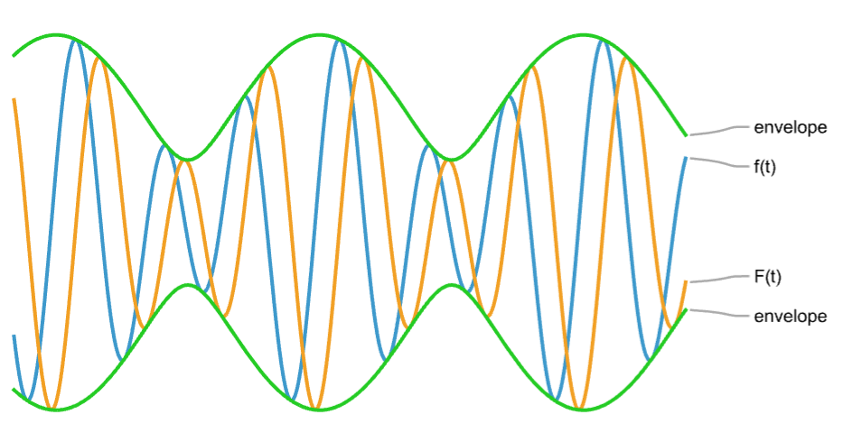
Wolfram Language code: InverseFourierTransform[H[ω], ω, t, FourierParameters -> {0, -2Pi}]

Wolfram Language code: Plot[%, {t, -4, 4}, PlotRange -> All]

Which is the same as:

Wolfram Language code: HilbertTransform[DiracDelta[t], t, t]

Its step response is:

Wolfram Language code:

InverseFourierTransform[H[ω] FourierTransform[UnitStep[t], t, ω, FourierParameters -> {0, -2 π}], ω, t, FourierParameters -> {0, -2 π}]

Wolfram Language code: Plot[{Abs@%, Arg@%}, {t, -10, 10}, PlotRange -> {-3, 2}, ...]

In signal processing, the Hilbert transform provides the imaginary component of the analytic representation of a real-valued signal :

Wolfram Language code:

u[t_] := Cos[2t + 3] + 2Cos[3t + 2];
Plot[u[t], {t, 0, 9}]

The Hilbert transform of is:

Wolfram Language code: U[t_] = HilbertTransform[u[t], t, t]

The analytic representation is:

Wolfram Language code: f[t_] = u[t] + I * U[t]

The envelope of an oscillating signal is a smooth curve outlining its extremes, and it is the magnitude of the analytic representation:

Wolfram Language code: Plot[{u[t], U[t], Abs[f[t]]}, {t, 0, 9}, Rule[...]]

Bedrosian's Theorem (1)

Suppose and have Fourier transforms and , respectively, where for with and for . Then .

Consider and as follows:

Wolfram Language code:

f[t_] := Cos[t / 2];
g[t_] := Cos[10t];

Verify the Fourier transform condition:

Wolfram Language code: Refine[FourierTransform[f[t], t, ω], ω > 0]

Wolfram Language code: Refine[FourierTransform[g[t], t, ω], ω > 0]

has a single spike at , while has a single spike at :

Wolfram Language code: ListPlot[{{{(1/2), Sqrt[2 π]}}, {{10, Sqrt[(π/2)]}}}, ...]

Any in between will suffice the hypothesis. Verify Bedrosian's theorem:

Wolfram Language code: HilbertTransform[f[t] * g[t], t, t]

Only the highpass signal needs to be transformed:

Wolfram Language code: f[t] * HilbertTransform[g[t], t, t]

Wolfram Language code: FullSimplify[% == %%]

Communications (1)

Consider a message signal:

Wolfram Language code:

m[t_] = (Cos[2Pi 5 t] + 2Cos[2Pi 7 t] + 1 / 2Cos[2 Pi 9 t]);
Plot[m[t], {t, -Pi / 2, Pi / 2}, ...]

Its Fourier transform:

Wolfram Language code: x[ω_] = FourierTransform[m[t], t, ω, FourierParameters -> {0, -2 * Pi}]

This provides the power spectrum:

Wolfram Language code: ListPlot[{{-9, (1/4)}, {-7, 1}, {-5, (1/2)}, {5, (1/2)}, {7, 1}, {9, (1/4)}}, ...]

Find the Hilbert transform of the message signal:

Wolfram Language code: Hm[s_] = HilbertTransform[m[t], t, s]

Wolfram Language code: Plot[Hm[t], {t, -Pi / 2, Pi / 2}, ...]

The power spectrum for the complex signal has only positive frequencies:

Wolfram Language code: FourierTransform[m[t] + I Hm[t], t, ω, FourierParameters -> {0, -2 * Pi}]

Wolfram Language code: ListPlot[{{9, (1/2)}, {7, 2}, {5, 1}}, ...]

Using as a message carrier, get the upper side band-suppressed carrier (USB-SC) and lower side band-suppressed carrier (LSB-SC):

Wolfram Language code:

USB[s_] = m[s]Cos[2Pi 35 s] - Hm[s]Sin[2 Pi 35 s];
LSB[s_] = m[s]Cos[2 Pi 35 s] + Hm[s]Sin[2 Pi 35 s];

Wolfram Language code: Plot[{USB[t], LSB[t]}, ...]

Their Fourier transforms:

Wolfram Language code: FourierTransform[{USB[t], LSB[t]}, t, ω, FourierParameters -> {0, -2 * Pi}]

They provide the power spectrum for both signals:

Wolfram Language code: ListPlot[{...}, AxesLabel -> {"Frequency", "Power"}, ...]

Properties & Relations (7)

For , the definite integral for HilbertTransform becomes:

Wolfram Language code: 1 / π * Integrate[Exp[-t ^ 2] / (s - t), {t, -∞, ∞}, PrincipalValue -> True]

Compare with HilbertTransform:

Wolfram Language code: HilbertTransform[Exp[-t ^ 2], t, s]

Linearity:

Wolfram Language code: HilbertTransform[a f[t] + b g[t], t, s]

Shifting:

Wolfram Language code: HilbertTransform[f[t + a], t, s]

Scaling:

Wolfram Language code: HilbertTransform[f[a t], t, s]

Time reversal:

Wolfram Language code: HilbertTransform[f[-t], t, s]

Hilbert transform of a Hilbert transform:

Wolfram Language code: HilbertTransform[HilbertTransform[f[t], t, s], s, t]

HilbertTransform and InverseHilbertTransform are mutual inverses:

Wolfram Language code: InverseHilbertTransform[HilbertTransform[f[t], t, s], s, t]

Wolfram Language code: HilbertTransform[InverseHilbertTransform[F[ t], t, s], s, t]

Wolfram Language code: HilbertTransform[1 / (t ^ 2 + 1), t, s]

Wolfram Language code: InverseHilbertTransform[%, s, t]

Possible Issues (1)

The result from an inverse Hilbert transform may not have the same form as the original:

Wolfram Language code: HilbertTransform[UnitStep[1 + t]UnitStep[1 - t], t, s]

Wolfram Language code: InverseHilbertTransform[%, s, t]

Interactive Examples (1)

In seismic data processing, important attributes can be obtained from the complex trace. For a seismic trace, compute its Hilbert transform:

Wolfram Language code:

u[t_] = Sin[2t + 3] + 2Sin[3t + 2] + 3Cos[2t + 3];
U[s_] = HilbertTransform[u[t], t, s];

The analytic representation is the complex trace :

Wolfram Language code: Manipulate[Show[...], {t, .0001, 6Pi}, Rule[...]]

Its envelope:

Wolfram Language code: Env[t_] = (u[t] ^ 2 + U[t] ^ 2) ^ (1 / 2)//FullSimplify

The envelope with its highest peaks marked:

Wolfram Language code:

Module[{...}, 
	CompoundExpression[...];
	Plot[{u[t], U[t], Env[t], -Env[t]}, ...]]

The instantaneous angular frequency is:

Wolfram Language code:

D[ArcTan[u[t], U[t]], t]//FullSimplify
Plot[%, {t, 0, 6π}]

Neat Examples (1)

Create a table of Hilbert transforms:

Wolfram Language code:

flist = {E ^ (I a t), E ^ (I / t), Exp[-t ^ 2], Sin[a t], Sin[6 t] / t, Sinc[t], DiracDelta[t + a], Log[Abs[t]], UnitStep[t], UnitBox[t]};

Wolfram Language code: Grid[Prepend[...], IconizedObject[«Grid options»]]//TraditionalForm

Top

HilbertTransform

Details and Options

Examples

Basic Examples (4)

Scope (29)

Basic Uses (4)

Elementary Functions (5)

Trigonometric Functions (4)

Powers and Algebraic Functions (5)

Generalized Functions (3)

Exponential and Logarithmic Functions (4)

Special Functions (2)

Formal Properties (1)

Numerical Evaluation (1)

Options (5)

AccuracyGoal (1)

Assumptions (1)

GenerateConditions (1)

PrecisionGoal (1)

WorkingPrecision (1)

Applications (5)

Basic Applications (1)

Signals and Systems (2)

Bedrosian's Theorem (1)

Communications (1)

Properties & Relations (7)

Possible Issues (1)

Interactive Examples (1)

Neat Examples (1)

See Also

Related Guides

History

Text

CMS

APA

BibTeX

BibLaTeX