

EstimatedPointNormals
EstimatedPointNormals[{p1,p2,…}]
estimates normal vectors for the points p1,p2,….
EstimatedPointNormals[mreg]
estimates normals vectors for the vertices of the mesh region mreg.
Details and Options
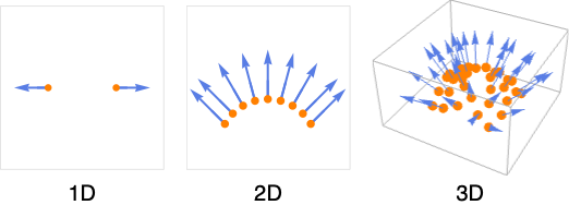
- EstimatedPointNormals is typically used to find hypersurface orientations from a set of points.
- EstimatedPointNormals[{p1,p2,…}] gives a list {n1,n2,…} where ni is the unit normal vector of pi.
- The pi in EstimatedPointNormals[{p1,p2,…}] can be lists of coordinates or explicit Point objects.
- A Method option can also be given. Possible Method settings include:
-
"PlaneFitting" plane fitting using nearest neighbors "FaceWeighted" face-weighted normals
Examples
open all close allBasic Examples (3)
Estimated normals of circle points:
pts = CirclePoints[20];
EstimatedPointNormals[pts]//ShallowGraphics[{Point[pts], Arrow /@ Transpose[{pts, pts + %}]}]Estimated normals of sphere points:
pts = SpherePoints[100];
EstimatedPointNormals[pts]//ShallowGraphics3D[{Point[pts], Arrow /@ Transpose[{pts, pts + %}]}]Generate a point cloud by randomly sampling a surface:
pts = RandomPoint[ResourceData["Stanford Bunny"], 20000];
Graphics3D[{AbsolutePointSize[1], Point[pts]}]
Visualize the estimated normals with lighting:
Graphics3D[{Point[pts, VertexNormals -> EstimatedPointNormals[pts]]}]Scope (2)
Basic Uses (1)
Estimated normals of points in 1D:
pts = {{-0.9}, {-1.0}, {-1.1}, {0.9}, {1.0}, {1.1}};
EstimatedPointNormals[pts]Graphics[{Point[Append[#, 0]& /@ pts], Arrow /@ Transpose[{Append[#, 0]& /@ pts, Append[#, 0]& /@ (pts + %)}]}]pts = RandomPoint[Circle[], 50];
EstimatedPointNormals[pts]//ShallowGraphics[{Point[pts], Arrow /@ Transpose[{pts, pts + %}]}]pts = RandomPoint[Sphere[], 100];
EstimatedPointNormals[pts]//ShallowGraphics3D[{Point[pts], Arrow /@ Transpose[{pts, pts + %}]}]pts = RandomPoint[Sphere[{0, 0, 0, 0, 0}], 120];
EstimatedPointNormals[pts]//ShallowSpecifications (1)
EstimatedPointNormals takes a set of points:
pts = {{-5, 0}, {-3, 0}, {-1, 0}, {1, 0}, {3, 0}, {5, 0}};EstimatedPointNormals[pts]Use a Point list:
EstimatedPointNormals[Point[pts]]Options (2)
Method (2)
Estimate point set normals by fitting a plane to each point's local neighborhood:
EstimatedPointNormals[CirclePoints[8], Method -> "PlaneFitting"]By default, mesh vertex normals are estimated using a weighted average of adjacent face normals:
mesh = [image];coords = MeshCoordinates[mesh];
normals = EstimatedPointNormals[mesh];Show[mesh, Graphics3D[{Arrow[Transpose[{coords, coords + normals}]]}]]pnormals = EstimatedPointNormals[mesh, Method -> "PlaneFitting"];Show[mesh, Graphics3D[{Arrow[Transpose[{coords, coords + pnormals}]]}]]This is equivalent to estimating the normals of the mesh coordinates directly:
EstimatedPointNormals[mesh, Method -> "PlaneFitting"] === EstimatedPointNormals[MeshCoordinates[mesh]]Applications (3)
Basic Applications (1)
Given a sufficiently dense sampling of a smooth surface, one can assume that samples near each other in space also lie near each other on the surface:
pts = Table[(2 + 2 / 3.5Sin[5 t]) * {Cos[t], Sin[t]}, {t, 0, 2 Pi, Pi / 40}];
nng = NearestNeighborGraph[pts, 4]
The local surface around each point is therefore sampled by the nearest neighborhood of the point:
ngs = NeighborhoodGraph[nng, pts[[#]]]& /@ {1, 10, 65}This local surface can be approximated by a plane fitted to its sample points:
fitPlane[p_] := Hyperplane[Eigensystem[Covariance[p]][[2, 2]], Mean[p]]
Show[#, Graphics[{Red, fitPlane[VertexList[#]]}]]& /@ ngs
The normals of these fitted planes can be used as an estimate of the normals of their corresponding points:
nls = Table[n = Eigensystem[Covariance[AdjacencyList[nng, pts[[pi]]]]][[2, 2]];
n * Sign[Dot[n, pts[[pi]]]], {pi, Length[pts]}];Graphics[Table[Arrow[{pts[[pi]], pts[[pi]] + nls[[pi]]}], {pi, Length[pts]}]]Point Cloud Rendering (1)
Render a point cloud using the estimated normals for lighting calculations:
pts = RandomPoint[ResourceData["Cow"], 6000];
Graphics3D[{AbsolutePointSize[1], Point[pts]}]Graphics3D[{Point[pts, VertexNormals -> EstimatedPointNormals[pts]]}]Compare the rendered point cloud to the ground truth model:
Graphics3D[{EdgeForm[], ResourceData["Cow"]}]Properties & Relations (2)
EstimatedPointNormals can generate normals for use in surface reconstruction:
pts = MeshCoordinates[ResourceData["Horse"]];
Graphics3D[{AbsolutePointSize[1], Point[pts]}]GradientFittedMesh[Point[pts, VertexNormals -> EstimatedPointNormals[pts]]]Normal vectors can be calculated directly using partial derivatives if the underlying function is known:
f[x_, y_] := Sin[x + Cos[y]]
fx = Subscript[∂, x]f[x, y];
fy = Subscript[∂, y]f[x, y];
fnormal[a_, b_] := {-fx, -fy, 1} /. {x -> a, y -> b};
farrow[x_, y_] := Arrow[{{x, y, f[x, y]}, {x, y, f[x, y]} + fnormal[x, y]}]
arrows = Table[farrow[x, y], {x, -Pi, Pi, Pi / 6}, {y, -Pi, Pi, Pi / 6}];

Show[Plot3D[f[x, y], {x, -Pi, Pi}, {y, -Pi, Pi}], Graphics3D[{Arrowheads[Small], arrows}], PlotRange -> All]
Interactive Examples (1)
Create an interactive example with draggable points to view the normals update in real time:
DynamicModule[{p = Table[(2 + 2 / 3.5 Sin[3 t]) * {Cos[t], Sin[t]}, {t, 0, 2 Pi, 0.15}]}, LocatorPane[Dynamic[p],
Graphics[{Dynamic[Arrow /@ Transpose[{p, p + EstimatedPointNormals[p]}]]}, PlotRange -> 4], Appearance -> "∘"]]Text
Wolfram Research (2022), EstimatedPointNormals, Wolfram Language function, https://reference.wolfram.com/language/ref/EstimatedPointNormals.html.
CMS
Wolfram Language. 2022. "EstimatedPointNormals." Wolfram Language & System Documentation Center. Wolfram Research. https://reference.wolfram.com/language/ref/EstimatedPointNormals.html.
APA
Wolfram Language. (2022). EstimatedPointNormals. Wolfram Language & System Documentation Center. Retrieved from https://reference.wolfram.com/language/ref/EstimatedPointNormals.html