

RegionFit
Details and Options
- RegionFit is also known as sample consensus model.
- RegionFit is typically used for fitting and reconstructing regions from a set of points.
- RegionFit[{p1,p2,…},"model"] finds a region that contains the most points pi by iteratively estimating parameters of the specified "model" from a set of points.
- Possible 2D "model" specifications include:
-

"Line" infinite line 
"Circle" circle - Possible 3D "model" specifications include:
-

"Line" infinite line 
"Circle" circle 
"Plane" plane 
"Sphere" sphere 
"Cylinder" cylinder 
"Cone" cone - RegionFit[Point[{p1,p2,…}]] is effectively equivalent to RegionFit[{p1,p2,…}].
- Vertex normals ni for points pi can be specified by Point[{p1,p2,…},VertexNormals{n1,n2,…}].
- RegionFit[{p1,p2,…},"model","prop"] returns the value of the fit property "prop".
- Possible fit properties "prop" include:
-
"BestFit" the best candidate model "Points" set of points "Inliers" points fitting the candidate model "Outliers" points not fitting the candidate model "DistanceVariance" variance of distances to the candidate model "Distances" distances to the best candidate model {prop1,prop2,…} several fit properties - The following options can be given:
-
ConfidenceLevel Automatic desired probability of outlier-free sample Method Automatic method to use PerformanceGoal $PerformanceGoal aspects of performance to try to optimize Tolerance Automatic numerical tolerance to use VertexNormals None vertex normals for points WorkingPrecision Automatic precision to use in computations - Possible settings for Method include:
-
"RANSAC" random sample consensus "LMEDS" least median of squares "MSAC" M-estimator sample consensus "RRANSAC" randomized RANSAC "RMSAC" randomized MSAC "MLESAC" maximum likelihood estimation sample consensus "PROSAC" progressive sample consensus
Examples
open all close allBasic Examples (2)
Find a circle that fits a set of points:
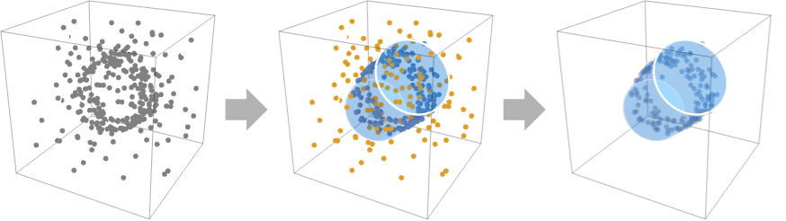
points = RandomPoint[Circle[{1, 2}, 3], 10];RegionFit[points, "Circle"]Graphics[{%, Point[points]}]A set of points with many outliers fitted by a cylinder:
data = Point[ {...}];RegionFit[data, "Cylinder"]Visualize the fitted region with the data:
Graphics3D[{data, RegionFit[data, "Cylinder"]}]Distribution of the distances of the data to the best‐fit cylinder:
Histogram[RegionFit[data, "Cylinder", "Distances"]]Scope (13)
Data (4)
RegionFit works on coordinates:
RegionFit[{{3, 9, 1}, {2, 5, 1}, {4, 7, 1}}, "Plane"]RegionFit[{Point[{3, 9, 1}], Point[{2, 5, 1}], Point[{4, 7, 1}]}, "Plane"]RegionFit[Point[{{3, 9, 1}, {2, 5, 1}, {4, 7, 1}}], "Plane"]Oriented collections of points:
RegionFit[Point[{{3, 9, 1}, {2, 5, 1}, {4, 7, 1}}, VertexNormals -> {{0, 0, 1}, {0, 0, 1}, {0, 0, 1}}], "Plane"]Models (7)
Obtain an InfiniteLine that best fits a set of points:
RegionFit[{{-24, -20}, {-24, -19}, {-25, -20}, {-80, -59}, {-76, -56}, {-95, -70}, {-83, -61}, {-95, -70}, {-46, -35}, {-58, -44}}, "Line"]RegionFit[{{88, 35}, {109, 51}, {117, 76}, {109, 101}, {88, 116}, {62, 116}, {40, 101}, {32, 76}, {40, 51}, {62, 35}}, "Circle"]InfiniteLine in 3D:
RegionFit[{{66, 55, 48}, {97, 74, 74}, {77, 62, 57}, {85, 67, 64}, {50, 45, 35}, {57, 49, 40}, {91, 71, 69}, {63, 53, 46}, {105, 79, 81}}, "Line"]RegionFit[IconizedObject[«data»], "Plane"]RegionFit[IconizedObject[«data»], "Sphere"]RegionFit[IconizedObject[«data»], "Cylinder"]Cone:
RegionFit[IconizedObject[«data»], "Cone"]Properties (2)
RegionFit gives the best fit region:
points = {{22, 22}, {3, 2}, {76, 75}, {48, 46}, {72, 72}, {95, 93}, {55, 54}, {8, 6}, {60, 62}, {78, 80}, {89, 89}, {0, 0}, {7, 43}, {100, 62}, {29, 85}, {61, 22}, {14, 53}, {13, 84}};RegionFit[points, "Line", "BestFit"]Distances of each point from the best fit region:
RegionFit[points, "Line", "Distances"]//NRegionFit[points, "Line", "DistanceVariance"]//Npoints = {{22, 22}, {3, 2}, {76, 75}, {48, 46}, {72, 72}, {95, 93}, {55, 54}, {8, 6}, {60, 62}, {78, 80}, {89, 89}, {0, 0}, {7, 43}, {100, 62}, {29, 85}, {61, 22}, {14, 53}, {13, 84}};{ℛ, inliers, outliers} = RegionFit[points, "Line", {"BestFit", "Inliers", "Outliers"}]Graphics[{Blue, Point[inliers], Red, Point[outliers], Gray, ℛ}]Options (6)
ConfidenceLevel (2)
The default gives an estimated 95% confidence that a sample will be chosen without outliers:
truth = Circle[{0.5, 0.5}, 0.3];
points = Join[RandomPoint[truth, 20], RandomReal[1, {200, 2}]];RegionFit[points, "Circle"]Graphics[{Point[points], LightGray, truth, Red, %}]RegionFit[points, "Circle", ConfidenceLevel -> 0.99]Graphics[{Point[points], LightGray, truth, Red, %}]RegionFit[points, "Circle", ConfidenceLevel -> 0.1]Graphics[{Point[points], LightGray, truth, Red, %}]Higher confidence levels tend to take more time while giving more accurate results:
truth = Circle[{0.5, 0.5}, 0.3];
points = Join[RandomPoint[truth, 100], RandomReal[1, {2000, 2}]];RegionFit[points, "Circle", ConfidenceLevel -> 0.1]//RepeatedTimingRegionFit[points, "Circle", ConfidenceLevel -> 0.99]//RepeatedTimingTolerance (1)
Use Tolerance to control the maximum distance of inliers:
points = Table[{x, x} + RandomReal[{-1, 1}15]{1, -1}, {x, 0, 100, 1}];
points//Short{ℛ1, inliers1} = RegionFit[points, "Line", {"BestFit", "Inliers"}, Tolerance -> 1];
{ℛ2, inliers2} = RegionFit[points, "Line", {"BestFit", "Inliers"}, Tolerance -> 15];
Graphics[{Gray, Point[points], Dashed, Blue, Point[inliers2], ℛ2, Red, Point[inliers1], ℛ1}]WorkingPrecision (3)
Compute the best-fit model using machine arithmetic:
points = Table[{x, x / 3}, {x, 2}];
RegionFit[points, "Line"]
Find the fit using exact numbers:
points = Table[{x, x / 3}, {x, 2}];
RegionFit[points, "Line", WorkingPrecision -> Infinity]
Find the fit using 30 digits of precision:
points = Table[{x, x / 3}, {x, 2}];
RegionFit[points, "Line", WorkingPrecision -> 30]
Applications (3)
Find a best-fit parametrized region for a set of points on a circle:
points = RandomPoint[Circle[{1, 2}, 3], 10];RegionFit[points, "Circle"]Graphics[{%, Point[points]}]points = RandomPoint[Circle[], 10];points = Join[RandomPoint[Circle[], 10], RandomVariate[NormalDistribution[], {10, 2}]];Find a best-fit parametrized region:
RegionFit[points, "Circle"]Visualize the fitted region with the data:
Graphics[{%, Point[points]}]Find the equation of a line passing through a set of points:
points = RandomPoint[Line[{{0, 0}, {1, 1}}], 10];RegionFit[points, "Line"]First[RegionConvert[%, "Implicit"]]Properties & Relations (1)
For near-perfect linear data, RegionFit and Fit produce equivalent fits using LeastSquares:
data = Table[{x, x / 2}, {x, 0, 10, 2}];Use Fit to find the equation of the line:
lineEq = Fit[data, {1, x}, x]Use RegionFit to find the line region:
lineRegion = RegionFit[data, "Line"]Show[Plot[lineEq /. x -> x, {x, 0, 10}, PlotRange -> Full], ListPlot[data], Graphics[lineRegion]]Fit minimizes the least squares error across all points, while RegionFit ignores outliers:
outlier = {2, 4};
odata = Append[data, outlier];lineEq = Fit[odata, {1, x}, x]
lineRegion = RegionFit[odata, "Line"]Show[Plot[lineEq /. x -> x, {x, 0, 10}, PlotRange -> Full], ListPlot[odata], Graphics[lineRegion]]Possible Issues (1)
RegionFit does not minimize error across all points:
points = {...};ListPlot[points, Prolog -> {RGBColor[0.880722, 0.611041, 0.142051], Thick, RegionFit[points, "Line"]}]ListPlot[points, PlotFit -> "Linear"]Neat Examples (1)
Visualize how the ConfidenceLevel affects the probability of finding the true region:
truth = Circle[{0.5, 0.5}, 0.3];
points = Join[RandomPoint[truth, 20], RandomReal[1, {160, 2}]];levels = {0.01, 0.33, 0.66, 0.99};
fits = Table[RegionFit[RandomSample[points, UpTo[Infinity]], "Circle", ConfidenceLevel -> cl], {cl, levels}, 50];
Graphics[{Point[points], Red, Thick, Opacity[0.04], #}, PlotRange -> {{0, 1}, {0, 1}}]& /@ fitsText
Wolfram Research (2021), RegionFit, Wolfram Language function, https://reference.wolfram.com/language/ref/RegionFit.html.
CMS
Wolfram Language. 2021. "RegionFit." Wolfram Language & System Documentation Center. Wolfram Research. https://reference.wolfram.com/language/ref/RegionFit.html.
APA
Wolfram Language. (2021). RegionFit. Wolfram Language & System Documentation Center. Retrieved from https://reference.wolfram.com/language/ref/RegionFit.html