

FluidViscosity
FluidViscosity[vars,pars,velocity]
yields fluid viscosity with variables vars, parameters pars and fluid velocity velocity.
Details
- FluidViscosity is an analysis function typically used to compute the viscosity of non-Newtonian flow such as lava or blood flow.
- FluidViscosity returns the apparent viscosity
 for non-Newtonian fluids and the dynamic viscosity
  for Newtonian fluids.
 - FluidViscosity is used by FluidViscousStress to compute the viscosity.
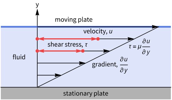
- Viscosity is a measure of a fluid's resistance to flow.
- FluidViscosity returns the fluid viscosity from a fluid's velocity vector velocity with variables of
 ,
,  and
and  in units of [
![TemplateBox[{InterpretationBox[, 1], {"m", , "/", , "s"}, meters per second, {{(, "Meters", )}, /, {(, "Seconds", )}}}, QuantityTF]](Files/FluidViscosity.en/7.png "TemplateBox[{InterpretationBox[, 1], {\"m\", , \"/\", , \"s\"}, meters per second, {{(, \"Meters\", )}, /, {(, \"Seconds\", )}}}, QuantityTF]") ], independent variables
], independent variables  in units of
  and time variable
  in units of [
![TemplateBox[{InterpretationBox[, 1], "s", seconds, "Seconds"}, QuantityTF]](Files/FluidViscosity.en/11.png "TemplateBox[{InterpretationBox[, 1], \"s\", seconds, \"Seconds\"}, QuantityTF]") ].
]. - FluidViscosity has the unit of [
![TemplateBox[{InterpretationBox[, 1], {"s", , "N", , "/", , {"m", ^, 2}}, second newtons per meter squared, {{(, {"Newtons", , "Seconds"}, )}, /, {(, {"Meters", ^, 2}, )}}}, QuantityTF]](Files/FluidViscosity.en/12.png "TemplateBox[{InterpretationBox[, 1], {\"s\", , \"N\", , \"/\", , {\"m\", ^, 2}}, second newtons per meter squared, {{(, {\"Newtons\", , \"Seconds\"}, )}, /, {(, {\"Meters\", ^, 2}, )}}}, QuantityTF]") ].
]. - FluidViscosity uses the same variables vars specification as FluidFlowPDEComponent.
- FluidViscosity uses the same parameter pars specification as FluidFlowPDEComponent.
- For dependent variables
 ,
,  and
and  given in vars, velocity components
  ,
,  and
and  need to be specified in velocity.
 - Typically, velocity is the result of solving a partial differential equation generated with FluidFlowPDEComponent.
- The specifics of the apparent viscosity
 depend on the chosen material model outlined in FluidFlowPDEComponent.
 - FluidViscosity supports custom non-Newtonian apparent viscosity models. »
Examples
open all close allBasic Examples (2)
FluidViscosity gives the dynamic viscosity for Newtonian fluids:
FluidViscosity[{{u[x, y], v[x, y], p[x, y]}, {x, y}}, <|"DynamicViscosity" -> μ|>, {𝒰[x, y], 𝒱[x, y]}]FluidViscosity returns the apparent viscosity for a non-Newtonian fluid:
FluidViscosity[{{u[x, y], v[x, y], p[x, y]}, {x, y}}, <|"MassDensity" -> ρ, "FluidDynamicsMaterialModel" -> <|"PowerLaw" -> <|"Exponent" -> n, "MinimalShearRate" -> Subscript[Overscript[γ, .], min], "ReferenceShearRate" -> Subscript[Overscript[γ, .], ref], "PowerLawViscosity" -> m|>|>|>, {𝒰[x, y], 𝒱[x, y]}]Scope (4)
FluidViscosity gives the viscosity specified through the Reynolds number ![]() :
:
FluidViscosity[{{u[x, y, z], v[x, y, z], w[x, y, z], p[x, y, z]}, {x, y, z}}, <|"ReynoldsNumber" -> ℛℯ|>, {𝒰[x, y, z], 𝒱[x, y, z], 𝒲[x, y, z]}]FluidViscosity supports axisymmetric flow:
FluidViscosity[{{rVel[r, z], 0, zVel[r, z], p[r, z]}, {r, θ, z}}, <|"MassDensity" -> ρ, "FluidDynamicsMaterialModel" -> <|"PowerLaw" -> <|"Exponent" -> n, "MinimalShearRate" -> Subscript[Overscript[γ, .], min], "ReferenceShearRate" -> Subscript[Overscript[γ, .], ref], "PowerLawViscosity" -> m|>|>, "RegionSymmetry" -> "Axisymmetric"|>, {ℛ[r, z], 0, 𝒵[r, z]}]Pressure may be an element of the velocity list but is not considered:
FluidViscosity[{{u[x, y], v[x, y], p[x, y]}, {x, y}}, <|"MassDensity" -> ρ, "FluidDynamicsMaterialModel" -> <|"PowerLaw" -> <|"Exponent" -> n, "MinimalShearRate" -> Subscript[Overscript[γ, .], min], "ReferenceShearRate" -> Subscript[Overscript[γ, .], ref], "PowerLawViscosity" -> m|>|>|>, {𝒰[x, y], 𝒱[x, y], 𝒫[x, y]}]Check that the viscosity is free of the pressure:
FreeQ[%, 𝒫[x, y]]Having the pressure in the velocity list is convenient such that the result of a FluidFlowPDEComponent simulation can directly be used. Set up the variables and parameters:
vars = {{u[x, y], v[x, y], p[x, y]}, {x, y}};
pars = <|"ReynoldsNumber" -> 1000|>;
Solve the fluid flow equations:
fluidFlowSolution = NDSolveValue[{FluidFlowPDEComponent[vars, pars] == {0, 0, 0}, DirichletCondition[{u[x, y] == 1, v[x, y] == 0}, y == 1], DirichletCondition[{u[x, y] == 0, v[x, y] == 0}, y < 1], DirichletCondition[p[x, y] == 0, x == 0 && y == 0]}, {u[x, y], v[x, y], p[x, y]}, {x, y}∈Rectangle[{0, 0}, {1, 1}], Method -> {"FiniteElement", "InterpolationOrder" -> {u -> 2, v -> 2, p -> 1}}]Compute the viscosity from the complete fluid flow solution:
FluidViscosity[vars, pars, fluidFlowSolution]Applications (2)
Compute the viscosity of the fluid flow of a non-Newtonian fluid in an opening channel by using the power law fluid flow model.
Ω = RegionUnion[Rectangle[{0, -1 / 2}, {5, 1 / 2}], Rectangle[{5, -3 / 2}, {30, 3 / 2}]];Set up variables, flow parameters and the non-Newtonian power law for parameters for the exponent and power law viscosity:
vars = {{u[x, y], v[x, y], p[x, y]}, {x, y}};
pars = <|"MassDensity" -> 1, "FluidDynamicsMaterialModel" -> <|"PowerLaw" -> <|"PowerLawExponent" -> 1 / 2, "PowerLawViscosity" -> 0.008838835|>|>
	|>;
Solve the PDE with an inflow profile given as {1/2,0} and with the outflow pressure set to 0. The walls are set up as no-slip walls:
fluidFlowResult = NDSolveValue[{FluidFlowPDEComponent[vars, pars] == {0, 0, 0}, DirichletCondition[
	{u[x, y] == 1 / 2, v[x, y] == 0}, x == 0], DirichletCondition[{u[x, y] == 0, v[x, y] == 0}, 0 < x < 30],
DirichletCondition[p[x, y] == 0, x == 30]}, vars[[1]], {x, y}∈Ω, Rule[...]]viscosity = FluidViscosity[vars, pars, fluidFlowResult]ContourPlot[viscosity, {x, y}∈Ω, PlotLegends -> Automatic]Compute the viscosity of a non-Newtonian fluid flow modeled with a custom-implemented power-law model. Define the custom apparent viscosity function:
apparentViscosity[vars_, pars_, data_] := Module[{strainRate, shearRate, viscosity, exponent}, viscosity = pars["FluidDynamicsMaterialModel"]["Custom"]["viscosity"];
	exponent = pars["FluidDynamicsMaterialModel"]["Custom"]["exponent"];
	strainRate = "StrainRate" /. data;
	shearRate = Sqrt[2 * ArrayDot[strainRate, strainRate, 2]];
viscosity * (shearRate) ^ (exponent - 1)]vars = {{u[x, y], v[x, y], p[x, y]}, {x, y}};pars = <|"MassDensity" -> 1, "FluidDynamicsMaterialModel" -> <|"Custom" -> <|"ApparentViscosityFunction" -> apparentViscosity, "viscosity" -> m, "exponent" -> n|>|>|>;Compute the apparent viscosity:
viscosity = FluidViscosity[vars, pars, {𝒰[x, y], 𝒱[x, y]}]Compare the result with the custom function:
strainRate = 1 / 2 * (Grad[{𝒰[x, y], 𝒱[x, y]}, {x, y}] + Transpose[Grad[{𝒰[x, y], 𝒱[x, y]}, {x, y}]]);
viscosity == apparentViscosity[{{𝒰[x, y], 𝒱[x, y], 𝒫[x, y]}, {x, y}}, pars, "StrainRate" -> strainRate]Text
Wolfram Research (2026), FluidViscosity, Wolfram Language function, https://reference.wolfram.com/language/ref/FluidViscosity.html.
CMS
Wolfram Language. 2026. "FluidViscosity." Wolfram Language & System Documentation Center. Wolfram Research. https://reference.wolfram.com/language/ref/FluidViscosity.html.
APA
Wolfram Language. (2026). FluidViscosity. Wolfram Language & System Documentation Center. Retrieved from https://reference.wolfram.com/language/ref/FluidViscosity.html