

FrequencySamplingFilterKernel
FrequencySamplingFilterKernel[{a1,…,ak}]
creates a finite impulse response (FIR) filter kernel using a frequency sampling method from amplitude values ai.
FrequencySamplingFilterKernel[{a1,…,ak},m]
creates an FIR filter kernel of type m.
Details and Options
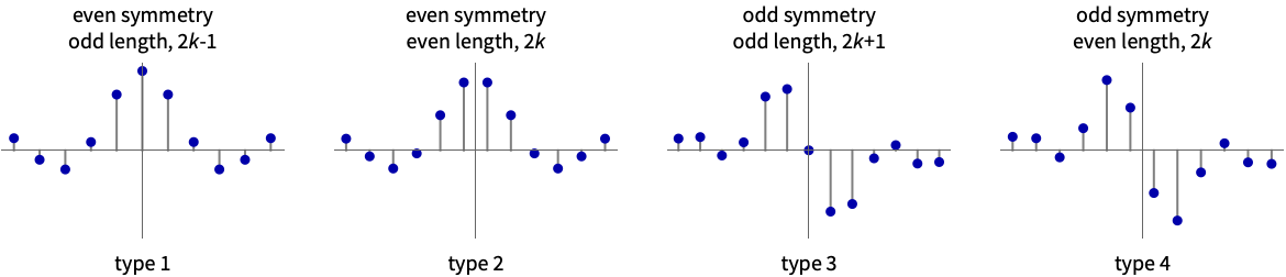
- Possible types m for FIR filters created for a list {a1,a2,…,ak} of amplitudes are:
- The default type is
 .
. - The frequency sampling method uniformly samples the frequency domain from 0 to
 .
. - FrequencySamplingFilterKernel by default uses a sampling of the frequency domain at integer multiples of
 , where
  is the length of the filter. With "Shifted"->True, the frequencies are shifted from 0 by
  . »
. » - Amplitude values should be non-negative. Typically, values ai=0 specify a stopband, and values ai=1 specify a passband.
- The kernel ker returned by FrequencySamplingFilterKernel can be used in ListConvolve[ker,data] to apply the filter to data.
- The following options can be given:
-
"Shifted" False whether the first frequency is offset from 0 WorkingPrecision MachinePrecision precision to use in internal computations
Examples
open all close allBasic Examples (1)
Scope (7)
A type 1 FIR kernel with even symmetry and odd length:
h = FrequencySamplingFilterKernel[{1, 1, 1, 0, 0, 0}, 1]Plot[Abs[ListFourierSequenceTransform[h, ω]], {ω, 0, π}]A type 2 FIR kernel with even symmetry and even length:
h = FrequencySamplingFilterKernel[{1, 1, 1, 0, 0, 0}, 2]Plot[Abs[ListFourierSequenceTransform[h, ω]], {ω, 0, π}]An odd-symmetry odd-length (type 3) bandpass kernel:
h = FrequencySamplingFilterKernel[{0, 0, 1, 1, 0, 0}, 3]Plot[Abs[ListFourierSequenceTransform[h, ω]], {ω, 0, π}, PlotRange -> All]An odd-symmetry even-length (type 4) highpass kernel:
h = FrequencySamplingFilterKernel[{0, 0, 0, 1, 1, 1}, 4]Plot[Abs[ListFourierSequenceTransform[h, ω]], {ω, 0, π}]A full-band differentiator FIR kernel:
h = FrequencySamplingFilterKernel[(Range[4] - 1 / 2) / 4, 4, "Shifted" -> True];
Plot[Abs[ListFourierSequenceTransform[h, ω]], {ω, 0, π}]
Create a filter from a random list of amplitude values:
a = RandomReal[1, 6]h = FrequencySamplingFilterKernel[a, 1];
Plot[Abs[ListFourierSequenceTransform[h, ω]], {ω, 0, π}, PlotRange -> All]Create a filter from an arbitrary function:
a = Table[1 / 2(Cos[x] + 1), {x, 0, π, π / 5}]//Nh = FrequencySamplingFilterKernel[a, 1];
Plot[Abs[ListFourierSequenceTransform[h, ω]], {ω, 0, π}, PlotRange -> All]Options (2)
"Shifted" (1)
By default, first frequency is sampled at 0:
a = FrequencySamplingFilterKernel[{1, 1, 0, 0}]Show[Plot[Abs[ListFourierSequenceTransform[a, x]], {x, 0, π}, PlotRange -> All], ListPlot[{{(0Pi / 14), 1}, {(4Pi / 14), 1}, {(8Pi / 14), 0}, {12Pi / 14, 0}}, Filling -> 0, PlotStyle -> {Red, PointSize[Large]}]]With "Shifted"->True, first frequency is offset from 0 by ![]() :
:
a = FrequencySamplingFilterKernel[{1, 1, 0, 0}, "Shifted" -> True]Show[Plot[Abs[ListFourierSequenceTransform[a, x]], {x, 0, π}, PlotRange -> All], ListPlot[{{(2Pi / 14), 1}, {(6Pi / 14), 1}, {(10Pi / 14), 0}, {Pi, 0}}, Filling -> 0, PlotStyle -> {Red, PointSize[Large]}]]WorkingPrecision (1)
By default, MachinePrecision is used:
h = FrequencySamplingFilterKernel[{1, 1, 1, 1, 0, 0, 0, 0}]Use 2-digit precision arithmetic:
g = Rationalize[#, 0]& /@ FrequencySamplingFilterKernel[{1, 1, 1, 1, 0, 0, 0, 0}, WorkingPrecision -> 2]Plot[Evaluate[{Abs[ListFourierSequenceTransform[h, x]], Abs[ListFourierSequenceTransform[g, x]]}], {x, 0, π}, PlotRange -> All]Applications (2)
Smooth data by convolving it with a lowpass filter kernel:
data = Table[ Sin[x] + RandomReal[.2], {x, 0, 2 Pi, 0.05}];
ker = FrequencySamplingFilterKernel[{1, 1, 0, 0, 0, 0, 0}];
ListLinePlot /@ {data, ListConvolve[ker, data, 7]}
Apply a derivative filter to rows of an image:
a = FrequencySamplingFilterKernel[{(1/8), (3/8), (5/8), (7/8)}, 4, "Shifted" -> True];
ImageConvolve[[image], {a}]//ImageAdjust
Properties & Relations (1)
Apply a window to an FIR filter to reduce ripple in its magnitude response:
fir = FrequencySamplingFilterKernel[{1, 1, 1, 0, 0, 0}]win = Array[BlackmanWindow, Length[fir], {-1 / 2, 1 / 2}];Plot[Evaluate[Abs[ListFourierSequenceTransform[#, x]]& /@ {fir, win fir}], {x, 0, π}]Text
Wolfram Research (2012), FrequencySamplingFilterKernel, Wolfram Language function, https://reference.wolfram.com/language/ref/FrequencySamplingFilterKernel.html.
CMS
Wolfram Language. 2012. "FrequencySamplingFilterKernel." Wolfram Language & System Documentation Center. Wolfram Research. https://reference.wolfram.com/language/ref/FrequencySamplingFilterKernel.html.
APA
Wolfram Language. (2012). FrequencySamplingFilterKernel. Wolfram Language & System Documentation Center. Retrieved from https://reference.wolfram.com/language/ref/FrequencySamplingFilterKernel.html