

LeastSquaresFilterKernel
LeastSquaresFilterKernel[{{ω1,…,ωk-1},{a1,…,ak}},n]
creates a k-band finite impulse response (FIR) filter kernel of length n designed using a least squares method, given the specified frequencies ωi and amplitudes ai.
LeastSquaresFilterKernel[{"type",spec},n]
uses the full filter specification {"type",spec}.
Details and Options
- LeastSquaresFilterKernel returns a numeric list of length n of the impulse response coefficients of an FIR filter that has the minimum mean-squared error.
- The impulse response of the filter is computed using the inverse discrete-time Fourier transform.
- In LeastSquaresFilterKernel[{"type",spec},n], filter specification can be any of the following:
-

{"Lowpass",ωc} lowpass filter with cutoff frequency ωc 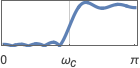
{"Highpass",ωc} highpass filter with cutoff frequency ωc 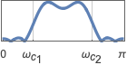
{"Bandpass",{ωc1,ωc2}} bandpass filter with passband from ωc1 to ωc2 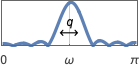
{"Bandpass",{{ω,q}}} bandpass filter with center frequency ω and quality factor q 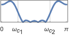
{"Bandstop",{ωc1,ωc2}} bandstop filter with stopband from ωc1 to ωc2 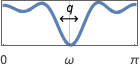
{"Bandstop",{{ω,q}}} bandstop filter with center frequency ω and quality factor q 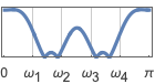
{"Multiband",{ω1,…,ωk-1},{a1,…,ak}} multiband filter specification with k bands 
{"Differentiator",ωc} differentiator filter with cutoff frequency ωc 
{"Hilbert",ωc} Hilbert filter with cutoff frequency ωc - If "type" is omitted, "Multiband" is assumed.
- Frequencies should be given in an ascending order such that 0≤ω1<ω2<…<ωk-1≤π.
- Amplitude value a1 corresponds to the frequency band 0 to ω1, and amplitude ak corresponds to the frequency band ωk-1 to π.
- Amplitude values should be non-negative. Typically, values ai=0 specify a stopband, and values ai=1 specify a passband.
- The quality factor q is defined as
 , with
  being the center frequency of a bandpass or bandstop filter. Higher values of q give narrower filters.
 - The kernel ker, returned by LeastSquaresFilterKernel, can be used in ListConvolve[ker,data] to apply the filter to data.
- The following option can be given:
-
WorkingPrecision MachinePrecision precision to use in internal computations
Examples
open all close allBasic Examples (2)
a = LeastSquaresFilterKernel[{"Lowpass", 1.2}, 15]Magnitude plot of the filter and its ideal lowpass prototype:
Plot[{Abs[ListFourierSequenceTransform[a, x]], Piecewise[{{1, 0 ≤ x ≤ 1.2}}]}, {x, 0, π}, PlotRange -> All, Exclusions -> False]BodePlot[ListZTransform[a, z], {0, π}, SamplingPeriod -> 1, PlotLayout -> "Magnitude", ScalingFunctions -> {"Linear", Automatic}, GridLines -> Automatic]spec = {{.5, 1, 2, 2.8}, {1, 0, 1, 0, 1}};
h = LeastSquaresFilterKernel[spec, 31]Magnitude plot of the filter and its "brickwall" specification:
Plot[Evaluate[{Abs[ListFourierSequenceTransform[h, x]], Piecewise[{#[[1]], #[[2, 1]] ≤ x ≤ #[[2, 2]]}& /@ Thread[{spec[[2]], Partition[Sort[Join[spec[[1]], {0., N[π]}]], 2, 1]}]]}], {x, 0, π}, Exclusions -> None, PlotRange -> All]Scope (6)
a = LeastSquaresFilterKernel[{"Highpass", 1.2}, 15]Plot[{Abs[ListFourierSequenceTransform[a, x]], UnitStep[x - 1.2]}, {x, 0, π}, PlotRange -> All, Exclusions -> None]ω1 = 1.;ω2 = 2.;
a = LeastSquaresFilterKernel[{"Bandpass", {ω1, ω2}}, 15]Plot[{Abs[ListFourierSequenceTransform[a, x]], UnitBox[x - 1.5]}, {x, 0, π}, PlotRange -> All, Exclusions -> None]Same filter using center frequency and quality factor specification:
ω0 = Sqrt[ω1 ω2];q = ω0 / (ω2 - ω1);
a = LeastSquaresFilterKernel[{"Bandpass", {{ω0, q}}}, 15];
Plot[{Abs[ListFourierSequenceTransform[a, x]], UnitBox[x - 1.5]}, {x, 0, π}, PlotRange -> All, Exclusions -> None]ω1 = 1.;ω2 = 2.;
a = LeastSquaresFilterKernel[{"Bandstop", {ω1, ω2}}, 21]Plot[{Abs[ListFourierSequenceTransform[a, x]], 1 - UnitBox[x - 1.5]}, {x, 0, π}, PlotRange -> All, Exclusions -> None]Same filter using center frequency and quality factor specification:
ω0 = Sqrt[ω1 ω2];q = ω0 / (ω2 - ω1);
a = LeastSquaresFilterKernel[{"Bandstop", {{ω0, q}}}, 21];
Plot[{Abs[ListFourierSequenceTransform[a, x]], 1 - UnitBox[x - 1.5]}, {x, 0, π}, PlotRange -> All, Exclusions -> None]a = LeastSquaresFilterKernel[{"Differentiator", 2}, 21]Plot[{Abs[ListFourierSequenceTransform[a, x]], x UnitStep[2 - x]}, {x, 0, π}, PlotRange -> All, Exclusions -> None]A full-band Hilbert FIR kernel:
a = LeastSquaresFilterKernel[{"Hilbert", π}, 21]Plot[Abs[ListFourierSequenceTransform[a, x]], {x, 0, π}, PlotRange -> All]Plot of the imaginary part of the filter:
Plot[Im@ListFourierSequenceTransform[a, x, -10], {x, -π, π}, PlotRange -> All]A half-band lowpass FIR kernel:
a = Chop@LeastSquaresFilterKernel[{"Lowpass", π / 2}, 15]Magnitude plot of the filter and the half-band frequency ![]() :
:
Plot[Abs[ListFourierSequenceTransform[a, x]], {x, 0, π}, PlotRange -> All, Epilog -> {Red, Dashed, Line[{{π / 2, 0}, {π / 2, 1}}]}]Convert the half-band lowpass filter to highpass:
b = Table[(-1)^i a[[i]], {i, 1, 15}]Magnitude plots of the two half-band filters:
Plot[Evaluate[Abs[ListFourierSequenceTransform[#, x]]& /@ {a, b}], {x, 0, π}, PlotRange -> All, Epilog -> {Red, Dashed, Line[{{π / 2, 0}, {π / 2, 1}}]}]Generalizations & Extensions (1)
Improve stopband attenuation by using a Blackman window:
n = 31;
fir = LeastSquaresFilterKernel[{"Lowpass", Pi / 2}, n];
fir2 = Array[BlackmanWindow, n, {-1 / 2, 1 / 2}] fir;BodePlot[{ListZTransform[fir, z], ListZTransform[fir2, z]}, {0, π}, SamplingPeriod -> 1, PlotLayout -> "Magnitude", GridLines -> Automatic, ScalingFunctions -> {"Linear", Automatic}]Applications (4)
Create a lowpass FIR filter with cutoff frequency of ![]() and length n=15:
and length n=15:
n = 15;
h = LeastSquaresFilterKernel[{"Lowpass", π / 5}, n]
Taper the filter using a Blackman window to improve stopband attenuation:
w = Array[BlackmanWindow, n, {-1 / 2, 1 / 2}];
fir = h w;fir / Total[fir]Log-magnitude plot of the power spectra of the two filters:
Plot[Evaluate[20Log10[Abs@ListFourierSequenceTransform[#, ω]]& /@ {h, %}], {ω, 0, π}, PlotRange -> {5, -125}, GridLines -> Automatic]Triple the length of the filter to match the bandwidth of the non-windowed sequence:
h2 = LeastSquaresFilterKernel[{"Lowpass", π / 5}, 3 n];
w2 = Array[BlackmanWindow, 3n, {-1 / 2, 1 / 2}];
fir = (h2 w2/Total[h2 w2]);
Plot[Evaluate[20Log10[Abs@ListFourierSequenceTransform[#, ω]]& /@ {h, fir}], {ω, 0, π}, PlotRange -> {5, -125}, GridLines -> Automatic]
Lowpass filtering of a dual-tone multi-frequency (DTMF) signal:
a = Mean[AudioGenerator[{"Sin", #}, 0.5, SampleRate -> 8000]& /@ {697, 1209}] + 0.05AudioGenerator["White", 0.5, SampleRate -> 8000]This shows the spectrum of the dual-tone signal:
Periodogram[a, PlotRange -> All]Create a windowed lowpass filter kernel with a cutoff frequency of 953 Hz for a sound sampled at 8000 Hz:
fir = LeastSquaresFilterKernel[{"Lowpass", 953 2π / 8000}, 71];
ker = Array[BlackmanWindow, Length[fir], {-.5, .5}]fir;b = Audio[{ListConvolve[ker, AudioData[a][[1]], 36, 0]}, SampleRate -> 8000]Here is the spectrum of the filtered signal:
Periodogram[b, PlotRange -> All]Create a list of Nyquist filters:
filters = LeastSquaresFilterKernel[{"Lowpass", π / #}, 31]& /@ {2, 3, 5};Plot[Evaluate[Abs[ListFourierSequenceTransform[#, x]]& /@ filters], {x, 0, π}, PlotLegends -> {2, 3, 5}]Take a derivative of the rows of an image:
h = LeastSquaresFilterKernel[{"Differentiator", π}, 8]ImageConvolve[[image], {h}]Properties & Relations (3)
Specifying the list of frequencies and amplitudes creates a multiband filter kernel:
LeastSquaresFilterKernel[{{1.2, 2}, {1, 0, 1}}, 31] === LeastSquaresFilterKernel[{"Multiband", {1.2, 2}, {1, 0, 1}}, 31]Increasing quality factors leads to narrower filters:
firs = LeastSquaresFilterKernel[{"Bandpass", {{1.0, #}}}, 33]& /@ {2 / 3, 1, 2};
BodePlot[ListZTransform[#, z]& /@ firs, {0, π}, SamplingPeriod -> 1, PlotLayout -> "Magnitude", ScalingFunctions -> {"Linear", Automatic}, GridLines -> Automatic, PlotLegends -> {"*q* = FractionBox[2, 3]", "*q* = 1", "*q* = 2"}]In a half-band filter of length ![]() , coefficients at positions
, coefficients at positions ![]() for positive integer values of
for positive integer values of ![]() are zero:
are zero:
n = 21;
a = LeastSquaresFilterKernel[{"Lowpass", (π/2)}, n]//ChopListPlot[a, AxesOrigin -> {(n + 1/2), 0}, Ticks -> None, PlotRange -> All, Filling -> 0]In a ![]() -band filter, coefficients at positions
-band filter, coefficients at positions ![]() are zero:
are zero:
k = 3;
a = LeastSquaresFilterKernel[{"Lowpass", (π/k)}, 21]//ChopListPlot[a, AxesOrigin -> {(n + 1/2), 0}, Ticks -> None, PlotRange -> All, Filling -> 0]Interactive Examples (1)
With[{chirp = Table[Cos[200. π t + 2400. π t ^ 2], {t, 0., 2., 1 / 8000.}],
w = Array[KaiserWindow, 91, {-1 / 2, 1 / 2}]},
Manipulate[audio = Audio[ListConvolve[w * LeastSquaresFilterKernel[{Range[1, 4] π / 5, {a1, a2, a3, a4, a5}}, 91], chirp, 1, 0], SampleRate -> 8000];
	Column[{Periodogram[audio, 4000, PlotRange -> {-60, 20}, ImageSize -> 240], audio}, Alignment -> Center]
, {{a1, 1}, 0.01, 10}, {{a2, 0.01}, 0.01, 10}, {{a3, 0.01}, 0.01, 10}, {{a4, 0.01}, 0.01, 10}, {{a5, 1}, 0.01, 10}, ContinuousAction -> True]]Text
Wolfram Research (2012), LeastSquaresFilterKernel, Wolfram Language function, https://reference.wolfram.com/language/ref/LeastSquaresFilterKernel.html (updated 2015).
CMS
Wolfram Language. 2012. "LeastSquaresFilterKernel." Wolfram Language & System Documentation Center. Wolfram Research. Last Modified 2015. https://reference.wolfram.com/language/ref/LeastSquaresFilterKernel.html.
APA
Wolfram Language. (2012). LeastSquaresFilterKernel. Wolfram Language & System Documentation Center. Retrieved from https://reference.wolfram.com/language/ref/LeastSquaresFilterKernel.html