FunctionInjective[f,x]
tests whether ![]() has at most one solution x∈Reals for each y.
has at most one solution x∈Reals for each y.
FunctionInjective[f,x,dom]
tests whether ![]() has at most one solution x∈dom.
has at most one solution x∈dom.
FunctionInjective[{f1,f2,…},{x1,x2,…},dom]
tests whether ![]() has at most one solution x1,x2,…∈dom.
has at most one solution x1,x2,…∈dom.
FunctionInjective[{funs,xcons,ycons},xvars,yvars,dom]
tests whether ![]() has at most one solution with xvars∈dom restricted by the constraints xcons for each yvars∈dom restricted by the constraints ycons.
has at most one solution with xvars∈dom restricted by the constraints xcons for each yvars∈dom restricted by the constraints ycons.


FunctionInjective
FunctionInjective[f,x]
tests whether ![]() has at most one solution x∈Reals for each y.
has at most one solution x∈Reals for each y.
FunctionInjective[f,x,dom]
tests whether ![]() has at most one solution x∈dom.
has at most one solution x∈dom.
FunctionInjective[{f1,f2,…},{x1,x2,…},dom]
tests whether ![]() has at most one solution x1,x2,…∈dom.
has at most one solution x1,x2,…∈dom.
FunctionInjective[{funs,xcons,ycons},xvars,yvars,dom]
tests whether ![]() has at most one solution with xvars∈dom restricted by the constraints xcons for each yvars∈dom restricted by the constraints ycons.
has at most one solution with xvars∈dom restricted by the constraints xcons for each yvars∈dom restricted by the constraints ycons.
Details and Options
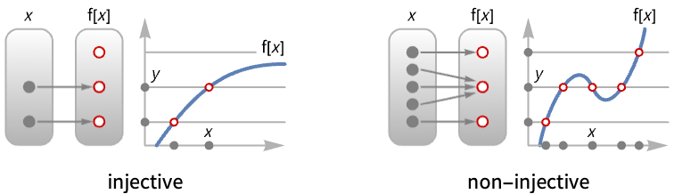
- An injective function is also known as one-to-one.
- A function
 is injective if for each
  there is at most one
  such that
  .
. - FunctionInjective[{funs,xcons,ycons},xvars,yvars,dom] returns True if the mapping
 is injective, where
  is the solution set of xcons and
  is the solution set of ycons.
 - If funs contains parameters other than xvars, the result is typically a ConditionalExpression.
- Possible values for dom are Reals and Complexes. If dom is Reals, then all variables, parameters, constants and function values are restricted to be real.
- The domain of funs is restricted by the condition given by FunctionDomain.
- xcons and ycons can contain equations, inequalities or logical combinations of these.
- The following options can be given:
-
Assumptions $Assumptions assumptions on parameters GenerateConditions True whether to generate conditions on parameters PerformanceGoal $PerformanceGoal whether to prioritize speed or quality - Possible settings for GenerateConditions include:
-
Automatic nongeneric conditions only True all conditions False no conditions None return unevaluated if conditions are needed - Possible settings for PerformanceGoal are "Speed" and "Quality".
Examples
open all close allBasic Examples (4)
Test injectivity of a univariate function over the reals:
FunctionInjective[E ^ x, x]Test injectivity over the complexes:
FunctionInjective[E ^ x, x, Complexes]Test injectivity of a polynomial mapping over the reals:
FunctionInjective[{x + y ^ 3, y - x ^ 5}, {x, y}]Test injectivity of a polynomial with symbolic coefficients:
FunctionInjective[x ^ 3 + a x + b, x]Scope (13)
FunctionInjective[x ^ 3 - x, x]Some values are attained more than once:
Plot[{x ^ 3 - x, 1 / 4}, {x, -2, 2}]Injectivity over a subset of the reals:
FunctionInjective[{x ^ 3 - x, x > 1}, x]For ![]() , each value is attained at most once:
, each value is attained at most once:
Plot[{x ^ 3 - x, 10}, {x, 1, 3}]Injectivity over the inverse image of a subset of the reals:
FunctionInjective[{x ^ 3 - x, True, y > 1 / 2}, x, y]Each value ![]() with
with ![]() is attained at most once:
is attained at most once:
Plot[{x ^ 3 - x, 1 / 2}, {x, -2, 2}]Injectivity over the complexes:
FunctionInjective[Log[x], x, Complexes]Each value is attained at most once:
Reduce[Log[x] == y, x]Injectivity over a subset of complexes:
FunctionInjective[{x ^ 3, Re[x] ≥ 0 && Im[x] ≥ 0}, x, Complexes]![]() is not injective over the whole complex plane:
is not injective over the whole complex plane:
FunctionInjective[x ^ 3, x, Complexes]Some values are attained more than once:
Reduce[x ^ 3 == 1, x]Injectivity from a subset of complexes to a subset of complexes:
FunctionInjective[{x ^ 2, Re[x] >= 0, Im[y] != 0}, x, y, Complexes]![]() is not injective for
is not injective for ![]() without the restriction on values:
without the restriction on values:
FunctionInjective[{x ^ 2, Re[x] >= 0}, x, y, Complexes]Some values with ![]() are attained more than once:
are attained more than once:
Reduce[x ^ 2 == -1 && Re[x] >= 0, x]Injectivity over the integers:
FunctionInjective[{Sin[x], Element[x, Integers]}, x]Injectivity of linear mappings:
A = {{1, 2, 3}, {4, 5, 6}, {7, 8, 9}};FunctionInjective[A.{x, y, z}, {x, y, z}]B = {{1, 2, 3}, {4, 5, 6}, {7, 8, 0}};FunctionInjective[B.{x, y, z}, {x, y, z}]A linear mapping is injective iff the rank of its matrix is equal to the dimension of its domain:
{MatrixRank[A], MatrixRank[B]}Injectivity of polynomial mappings ![]() :
:
FunctionInjective[{x ^ 2 + 2x, x ^ 3 - x}, x]Each value is attained at most once:
ParametricPlot3D[{{x, x ^ 2 + 2x, x ^ 3 - x}, {x, 3, 0}}, {x, -3, 3}]This mapping is not injective:
FunctionInjective[{x ^ 2 + x, x ^ 3 - x}, x]Some values are attained more than once:
ParametricPlot3D[{{x, x ^ 2 + x, x ^ 3 - x}, {x, 0, 0}}, {x, -2, 2}]Injectivity of polynomial mappings ![]() :
:
FunctionInjective[{x ^ 3 - 3x y ^ 2, 3x ^ 2y - y ^ 3}, {x, y}]The mapping, equal to the real and imaginary parts of ![]() , is injective in the non-negative quadrant:
, is injective in the non-negative quadrant:
FunctionInjective[{{x ^ 3 - 3x y ^ 2, 3x ^ 2y - y ^ 3}, x ≥ 0 && y ≥ 0}, {x, y}]Injectivity of polynomial mappings ![]() :
:
FunctionInjective[{x + y ^ 3, y - x ^ 5}, {x, y}, Complexes]The Jacobian determinant of an injective complex polynomial mapping must be constant:
Det[D[{x + y ^ 3, y - x ^ 5}, {{x, y}}]]The Jacobian conjecture states that the reverse implication is true:
Det[D[{x - (x + y / 27) ^ 3, y + (3 x + y / 9) ^ 3}, {{x, y}}]]Indeed, this polynomial mapping with a constant Jacobian is injective:
FunctionInjective[{x - (x + y / 27) ^ 3, y + (3 x + y / 9) ^ 3}, {x, y}, Complexes]Injectivity of a real polynomial with symbolic parameters:
FunctionInjective[x ^ 3 + a x ^ 2 + b x + c, x]Injectivity of a real polynomial mapping with symbolic parameters:
FunctionInjective[{x + a y ^ 3, y + b x ^ 3}, {x, y}]Options (4)
Assumptions (1)
FunctionInjective is unable to decide injectivity of ![]() for arbitrary
for arbitrary ![]() :
:
FunctionInjective[BesselI[n, x], x]With ![]() assumed to be an odd integer, FunctionInjective succeeds:
assumed to be an odd integer, FunctionInjective succeeds:
FunctionInjective[BesselI[n, x], x, Assumptions -> Element[(n + 1) / 2, Integers]]Plot[Evaluate[Table[BesselI[n, x], {n, 1, 9, 2}]], {x, -10, 10}]GenerateConditions (2)
By default, FunctionInjective may generate conditions on symbolic parameters:
FunctionInjective[E ^ x + a x, x]With GenerateConditionsNone, FunctionInjective fails instead of giving a conditional result:
FunctionInjective[E ^ x + a x, x, GenerateConditions -> None]This returns a conditionally valid result without stating the condition:
FunctionInjective[E ^ x + a x, x, GenerateConditions -> False]By default, all conditions are reported:
FunctionInjective[a x, x, Complexes]With GenerateConditionsAutomatic, conditions that are generically true are not reported:
FunctionInjective[a x, x, Complexes, GenerateConditions -> Automatic]PerformanceGoal (1)
Use PerformanceGoal to avoid potentially expensive computations:
FunctionInjective[x ^ 5 + a x ^ 4 + b x ^ 3 + c x ^ 2 + d x, x, PerformanceGoal -> "Speed"]The default setting uses all available techniques to try to produce a result:
FunctionInjective[x ^ 5 + a x ^ 4 + b x ^ 3 + c x ^ 2 + d x, x]Applications (17)
Basic Applications (8)
FunctionInjective[Cos[x], x]![]() is not injective, because the value
is not injective, because the value ![]() is attained more than once:
is attained more than once:
Plot[{Cos[x], 1 / 2}, {x, -2Pi, 2Pi}]FunctionInjective[ArcTan[x], x]Each value is attained at most once:
Plot[{ArcTan[x], 1, 2}, {x, -5, 5}]Check injectivity of ![]() in its real domain:
in its real domain:
FunctionInjective[Sqrt[x], x]![]() is injective in its real domain
is injective in its real domain ![]() :
:
Plot[{Sqrt[x], 1, -1}, {x, -10, 10}]Check injectivity of Clip[x] over unrestricted reals:
FunctionInjective[Clip[x], x]Values ![]() and
and ![]() are attained more than once on, respectively, [-∞,-1] and [1, ∞]:
are attained more than once on, respectively, [-∞,-1] and [1, ∞]:
Plot[Clip[x], {x, -2, 2}]Clip[x] restricted to the interval [-1, 1] is injective:
FunctionInjective[{Clip[x], -1 ≤ x ≤ 1}, x]A function is injective if any horizontal line intersects its graph at most once:
FunctionInjective[Erf[x], x]Manipulate[Plot[{Erf[x], a}, ...], {{a, 0.5}, -1.5, 1.5}]If a horizontal line intersects the graph more than once, the function is not injective:
FunctionInjective[(3x ^ 3 + 7x ^ 2) / (2x ^ 3 + 1), x]Manipulate[Plot[{(3x ^ 3 + 7x ^ 2) / (2x ^ 3 + 1), a}, ...], {{a, 3}, -3, 4}]Periodic functions are not injective:
FunctionInjective[Tan[x], x]Use FunctionPeriod to check whether a function is periodic:
FunctionPeriod[Tan[x], x]A periodic function attains each value infinitely many times:
Plot[{Tan[x], 1}, {x, -5 / 2Pi, 5 / 2Pi}]Functions whose derivative has a fixed positive or negative sign are injective:
FunctionInjective[Sin[x] + 2x, x]Use FunctionSign to find the sign of a derivative:
FunctionSign[D[Sin[x] + 2x, x], x]The function is strictly increasing, and hence injective:
Plot[Sin[x] + 2x, {x, -10, 10}]Integrals of functions that have a fixed positive or negative sign are injective:
f = Integrate[Cos[t] ^ 2 + E ^ -t, {t, 0, x}]FunctionInjective[f, x]Plot[f, {x, 0, 10}]Integrate a positive piecewise function for argument values in [0,2]:
g = Integrate[TriangleWave[t] + 5 / 4, {t, 0, x}, Assumptions -> 0 ≤ x ≤ 2]The integral is injective for 0≤x≤2:
FunctionInjective[{g, 0 ≤ x ≤ 2}, x]Plot[g, {x, 0, 2}]Injective functions do not need to be continuous or monotonic:
f = Piecewise[{{x, Sin[π x] ≥ 0}, {2Ceiling[x] - 1 - x, Sin[π x] < 0}}];FunctionInjective[{f, 0 < x < 10}, x]Plot[f, {x, 0, 10}, ImageSize -> Small]A continuous injective function does not need to be monotonic:
FunctionInjective[1 / x, x]Plot[1 / x, {x, -2, 2}]The function is continuous, but its domain is not a connected set:
FunctionContinuous[{1 / x, x ≠ 0}, x]FunctionDomain[1 / x, x]Check injectivity of a mapping ![]() :
:
FunctionInjective[{x^2 + y^2, x - y}, {x, y}]A part of the ParametricPlot has been covered twice:
ParametricPlot[{x^2 + y^2, x - y}, {x, -1, 1}, {y, 0, 1}, Mesh -> Full]For positive ![]() and
and ![]() , the mapping is injective:
, the mapping is injective:
FunctionInjective[{{x^2 + y^2, x - y}, x > 0 && y > 0}, {x, y}]Each point of the ParametricPlot is covered once:
ParametricPlot[{x^2 + y^2, x - y}, {x, 0, 1}, {y, 0, 1}, Mesh -> Full]Here, the point {0,0} is clearly covered multiple times:
ParametricPlot[{x^2 - y^2, x - y}, {x, -1, 1}, {y, -1, 1}, Mesh -> Full]These are all the ![]() and
and ![]() that map to {0,0}:
that map to {0,0}:
Reduce[{x^2 - y^2, x - y} == {0, 0}, {x, y}]Apart from that, the mapping is injective:
FunctionInjective[{{x^2 - y^2, x - y}, x ≠ y}, {x, y}]Solving Equations & Inequalities (4)
![]() is injective if for any value of
is injective if for any value of ![]() , the equation
, the equation ![]() has at most one solution for
has at most one solution for ![]() :
:
FunctionInjective[ArcTan[(x ^ 5 + 3x ^ 3 + 2x) / (4x ^ 4 + 4)], x]Plot[{ArcTan[(x ^ 5 + 3x ^ 3 + 2x) / (4x ^ 4 + 4)], 1, 2}, {x, -10, 10}]Solve[ArcTan[(x ^ 5 + 3x ^ 3 + 2x) / (4x ^ 4 + 4)] == 1, x, Reals]Solve[ArcTan[(x ^ 5 + 3x ^ 3 + 2x) / (4x ^ 4 + 4)] == 2, x, Reals]There is at most one solution of ![]() :
:
Solve[ArcTan[(x ^ 5 + 3x ^ 3 + 2x) / (4x ^ 4 + 4)] == y, x, Reals]f = {x ^ 3, x - y ^ 2}FunctionInjective[f, {x, y}]The equation ![]() has two solutions:
has two solutions:
Solve[f == {2, 1}, {x, y}, Reals]The restriction of ![]() to
to ![]() is injective:
is injective:
FunctionInjective[{f, y ≥ 0}, {x, y}]The equation ![]() has at most one solution with
has at most one solution with ![]() :
:
Solve[f == {u, v} && y ≥ 0, {x, y}, Reals]Any injective function ![]() has an inverse function:
has an inverse function:
f := Function[x, ConditionalExpression[Erf[x] ^ 3, Element[x, Reals]]]FunctionInjective[f[x], x]Plot[f[x], {x, -3, 3}]The domain of the inverse function is the range of ![]() :
:
g = InverseFunction[f]Plot[g[y], {y, -1, 1}]A differentiable function with a nonzero derivative, defined on a connected set, is injective:
f = Log[x ^ 2 + 1]The derivative of ![]() is positive for
is positive for ![]() :
:
df = D[f, x]FunctionSign[{df, x > 0}, x]FunctionInjective[{f, x > 0}, x]The inverse function of ![]() satisfies the equation
satisfies the equation ![]() :
:
invf = DSolveValue[{g'[y] == 1 / (df /. x -> g[y]), g[f /. x -> 1] == 1}, g[y], y]Check that the result is indeed the inverse function of ![]() for
for ![]() :
:
Simplify[{invf /. y -> f, f /. x -> invf}, x > 0 && Element[y, Reals]]Probability & Statistics (2)
The CDF of a distribution with a strictly positive PDF is injective:
pdf = PDF[NormalDistribution[], x]FunctionSign[pdf, x]Plot[pdf, {x, -5, 5}]cdf = CDF[NormalDistribution[], x]FunctionInjective[cdf, x]Plot[cdf, {x, -5, 5}]SurvivalFunction and Quantile are injective as well:
sf = SurvivalFunction[NormalDistribution[], x]FunctionInjective[sf, x]Plot[sf, {x, -5, 5}]qf = Quantile[NormalDistribution[], x]FunctionInjective[qf, x]Plot[qf, {x, 0, 1}]Calculus (3)
Compute ![]() by change of variables:
by change of variables:
e = Exp[-(x ^ 3 + y ^ 2) ^ 2] / (y ^ 6 + 1)x ^ 2y ^ 2;If ![]() is an injective mapping, then
is an injective mapping, then ![]() :
:
f[{u_, v_}] := 1 / 9Exp[-u ^ 2] / (v ^ 2 + 1)
g = {x ^ 3 + y ^ 2, y ^ 3};FunctionInjective[g, {x, y}]f[g]Det[D[g, {{x, y}}]] === eFind the range of ![]() to determine the integration bounds:
to determine the integration bounds:
FunctionRange[g, {x, y}, {u, v}]Integrate[f[{u, v}], {u, -Infinity, Infinity}, {v, -Infinity, Infinity}]Compute the original integral directly:
Integrate[e, {x, -Infinity, Infinity}, {y, -Infinity, Infinity}]Compute the surface area of a ball with radius ![]() using a rational parametrization:
using a rational parametrization:
f = {(2 r (1 - t^2) u/(1 + t^2) (1 + u^2)), (4 r t u/(1 + t^2) (1 + u^2)), (r (1 - u^2)/1 + u^2)};ParametricPlot3D[Evaluate[f /. r -> 1], {t, -50, 50}, {u, 0, 50}, ...]Check that the parametrization is injective:
FunctionInjective[{f, u > 0}, {t, u}, Assumptions -> r > 0]The surface area is equal to the integral of square root of Gram determinant of ![]() :
:
df = D[f, {{t, u}}];Integrate[Sqrt[Det[Transpose[df].df]], {u, 0, ∞}, {t, -∞, ∞}, Assumptions -> r > 0]Integrate ![]() over the "eight surface" using a rational parametrization:
over the "eight surface" using a rational parametrization:
f = {(4 (1 - t^2) u (1 - u^2)/(1 + t^2) (1 + u^2)^2), (8 t u (1 - u^2)/(1 + t^2) (1 + u^2)^2), (2 u/1 + u^2)};
g[{x_, y_, z_}] := E ^ (x + y + z)ParametricPlot3D[f, {t, 0, 50}, {u, -50, 50}, ...]Check that the parametrization is injective outside a one-dimensional set:
FunctionInjective[{f, t > 0 && u ≠ 0 && t ^ 2 ≠ 1 && u ^ 2 ≠ 1}, {t, u}]df = D[f, {{t, u}}];NIntegrate[g[f]Sqrt[Det[Transpose[df].df]], {t, 0, ∞}, {u, -∞, ∞}]Compare with the value computed using the implicit description of the "eight surface":
reg = ImplicitRegion[x ^ 2 + y ^ 2 - 4z ^ 2 + 4z ^ 4 == 0, {x, y, z}];NIntegrate[g[v], Element[v, reg]]Properties & Relations (3)
![]() is injective iff the equation
is injective iff the equation ![]() has at most one solution for each
has at most one solution for each ![]() :
:
FunctionInjective[x ^ 2 + x + 1, x]FunctionInjective[x ^ 3 + x + 1, x]Use Solve to find the solutions:
Solve[x ^ 2 + x + 1 == y, x, Reals]Solve[x ^ 3 + x + 1 == y, x, Reals]A real univariate continuous function on a connected set is injective iff it is monotonic:
FunctionInjective[{Sin[x], 0 ≤ x ≤ Pi}, x]FunctionInjective[{Cos[x], 0 ≤ x ≤ Pi}, x]Plot[{Sin[x], Cos[x]}, {x, 0, Pi}]Use FunctionMonotonicity to determine the monotonicity of a function:
FunctionMonotonicity[{Sin[x], 0 ≤ x ≤ Pi}, x]FunctionMonotonicity[{Cos[x], 0 ≤ x ≤ Pi}, x]A complex polynomial mapping is injective iff it has a polynomial inverse:
F = {x - (x + y / 27) ^ 3, y + (3 x + y / 9) ^ 3};FunctionInjective[F, {x, y}, Complexes]Use Solve to find the polynomial inverse:
G = {x, y} /. Solve[{u, v} == {x - (x + y / 27) ^ 3, y + (3 x + y / 9) ^ 3}, {x, y}][[1]]Verify that ![]() is a two-sided inverse of
is a two-sided inverse of ![]() :
:
Expand[G /. Thread[{u, v} -> F]]Expand[F /. Thread[{x, y} -> G]]Possible Issues (1)
FunctionInjective determines the real domain of functions using FunctionDomain:
FunctionInjective[Cosh[Sqrt[x]], x]![]() is injective in the real domain reported by FunctionDomain:
is injective in the real domain reported by FunctionDomain:
FunctionDomain[Cosh[Sqrt[x]], x]Plot[{Cosh[Sqrt[x]], 7}, {x, 0, 10}]![]() is real valued and not injective over the whole reals:
is real valued and not injective over the whole reals:
Plot[{Cosh[Sqrt[x]], -1 / 2}, {x, -20, 10}]All subexpressions of ![]() need to be real valued for a point to belong to the real domain of
need to be real valued for a point to belong to the real domain of ![]() :
:
Refine[Element[Sqrt[x], Reals], x < 0]Text
Wolfram Research (2020), FunctionInjective, Wolfram Language function, https://reference.wolfram.com/language/ref/FunctionInjective.html.
CMS
Wolfram Language. 2020. "FunctionInjective." Wolfram Language & System Documentation Center. Wolfram Research. https://reference.wolfram.com/language/ref/FunctionInjective.html.
APA
Wolfram Language. (2020). FunctionInjective. Wolfram Language & System Documentation Center. Retrieved from https://reference.wolfram.com/language/ref/FunctionInjective.html