Wolfram Language & System Documentation Center

Quantile

Quantile[data,p]

gives the estimate of the p quantile of data.

Quantile[data,{p₁,p₂,…}]

gives a list of quantiles p₁,p₂,….

Quantile[data,p,{{a,b},{c,d}}]

uses the quantile definition specified by parameters a, b, c, d.

Quantile[dist,p]

gives a quantile of the distribution dist.

Details

Quantile is also known as value at risk (VaR) or fractile.
When VectorQ data is sorted as , the quantile estimate is given by .

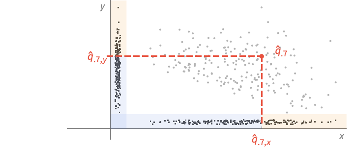
For MatrixQ data, the quantile is computed for each column vector with Quantile[{{x₁,y₁,…},{x₂,y₂,…},…},p] equivalent to {Quantile[{x₁,x₂,…},p],Quantile[{y₁,y₂,…},p]}. »

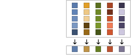
For ArrayQ data, quantile is equivalent to ArrayReduce[Quantile,data,1]. »

Quantile[ ${x_1,...,x_n}$ ,p,{{a,b},{c,d}}] is given by with r=a+(n+b)p, ⌊r⌋= Floor[r], ⌈r⌉=Ceiling[r] and =FractionalPart[r]. The indices are taken to be 1 or n if they are out of range. »
Common choices of parameters {{a,b},{c,d}} include:

	{{0,0},{1,0}}	inverse empirical CDF (default)
	{{0,0},{0,1}}	linear interpolation (California method)
	{{1/2,0},{0,0}}	element numbered closest to p n
	{{1/2,0},{0,1}}	linear interpolation (hydrologist method)
	{{0,1},{0,1}}	mean‐based estimate (Weibull method)
	{{1,-1},{0,1}}	mode‐based estimate
	{{1/3,1/3},{0,1}}	median‐based estimate
	{{3/8,1/4},{0,1}}	normal distribution estimate

The default choice of parameters is {{0,0},{1,0}}.
About 10 different choices of parameters are in use in statistical work.
Quantile[list,p] always gives a result equal to an element of list.
The same is true whenever d is 0.
When d is 1, Quantile is piecewise linear as a function of p.
Median[data] is equivalent to Quantile[data,1/2,{{1/2,0},{0,1}}].
The data can have the following additional forms and interpretations:

	Association	the values (the keys are ignored) »
	SparseArray	as an array, equivalent to Normal[data] »
	QuantityArray	quantities as an array »
	WeightedData	based on the underlying EmpiricalDistribution »
	EventData	based on the underlying SurvivalDistribution »
	TimeSeries, TemporalData, …	vector or array of values (the time stamps ignored) »
	Image,Image3D	RGB channel's values or grayscale intensity value »
	Audio	amplitude values of all channels »
	DateObject, TimeObject	list of dates or list of times »

Quantile[dist,p] is equivalent to InverseCDF[dist,p].
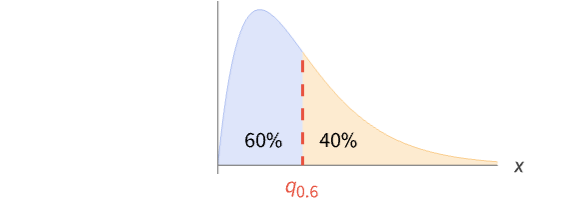
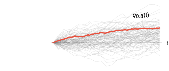
Quantile[dist,p] is the minimum of the set of number(s) such that Probability[x≤,xdist]≥p and Probability[x≥,xdist]≥p. »

For a random process proc, the quantile function can be computed for slice distribution at time t, SliceDistribution[proc,t], as Quantile[SliceDistribution[proc,t], p]. »

The value p can be symbolic or any number between 0 and 1. »

Examples

open all close all

Basic Examples (7)

Find the halfway value of a list:

Wolfram Language code: Quantile[{1, 2, 3, 4, 5, 6, 7}, 1 / 2]

Find the 20% and 80% quantiles of a list:

Wolfram Language code: Quantile[{1, 2, 3, 4, 5, 6, 7}, {0.2, 0.8}]

Find the top percentile of a list:

Wolfram Language code: Quantile[Range[100], .99]

Quantile of a list of dates:

Wolfram Language code: RandomDate[4]

Wolfram Language code: Quantile[%, .3]

The q quantile for a normal distribution:

Wolfram Language code: Quantile[NormalDistribution[μ, σ], q]

Quantile function for a continuous univariate distribution:

Wolfram Language code: Plot[Table[Quantile[BetaDistribution[1 / 2, β], q], {β, {1 / 4, 1 / 2, 1}}]//Evaluate, {q, 0, 1}, Filling -> Axis]

Quantile function for a discrete univariate distribution:

Wolfram Language code: 𝒟 = PoissonDistribution[5];

Wolfram Language code: DiscretePlot[Quantile[𝒟, p], {p, CDF[𝒟, Range[0, 10]]}, ExtentSize -> Left, ExtentMarkers -> {"Empty", "Filled"}]

Scope (33)

Basic Uses (7)

Quantile works with any real numeric quantities:

Wolfram Language code: Quantile[{E, Pi, Sqrt[2], Sqrt[3]}, 1 / 4]

Obtain results at any precision:

Wolfram Language code: Quantile[N[{5, 10, 4, 25, 2, 1}, 30], 2 / 3]

Compute results using other parametrizations:

Wolfram Language code: Quantile[{5, 10, 4, 25, 2, 1}, 1 / 5]

Wolfram Language code: Quantile[{5, 10, 4, 25, 2, 1}, 1 / 5, {{1 / 2, 0}, {0, 1}}]

Find quantiles for WeightedData:

Wolfram Language code: Quantile[WeightedData[{1, 2, 3}, {3, 7, 4}], 0.4]

Wolfram Language code:

data = {8, 3, 5, 4, 9, 0, 4, 2, 2, 3};
weights = {0.15, 0.09, 0.12, 0.10, 0.16, 0., 0.11, 0.08, 0.08, 0.09};

Wolfram Language code: Quantile[WeightedData[data, weights], 0.4]

Find quantiles for EventData:

Wolfram Language code:

e = {1.0, 2.1, 3.2, 4.5, 5.7};
ci = {0, 0, 0, 1, 0};

Wolfram Language code: Quantile[EventData[e, ci], 0.4]

Find a quantile for TimeSeries:

Wolfram Language code:

Quantile[TemporalData[TimeSeries, {{{2.3, 1.2, 6.7, 5.8, 7.1, 4.6}}, {{0, 5, 1}}, 1, {"Discrete", 1}, 
  {"Discrete", 1}, 1, {}}, False, 10.], 0.4]

The quantile depends only on the values:

Wolfram Language code:

Quantile[TemporalData[TimeSeries, {{{2.3, 1.2, 6.7, 5.8, 7.1, 4.6}}, {{0, 5, 1}}, 1, {"Discrete", 1}, 
  {"Discrete", 1}, 1, {}}, False, 10.]["Values"], 0.4]

Find a quantile for data involving quantities:

Wolfram Language code: data = Quantity[RandomReal[1, 6], "Meters"]

Wolfram Language code: Quantile[data, 0.3]

Array Data (6)

Find quantiles of elements in each column:

Wolfram Language code: Quantile[{{1, 2Pi}, {2, Pi}, {3, 3Pi}}, 1 / 3]

Find multiple quantiles of elements in each column:

Wolfram Language code: Quantile[{{1, 2Pi}, {2, Pi}, {3, 3Pi}}, {1 / 3, 4 / 5}]

The quantile for a tensor gives columnwise standard deviations at the first level:

Wolfram Language code: Quantile[RandomReal[1, {10, 4, 3}], .2]

Compute results for a large vector or matrix:

Wolfram Language code: Quantile[RandomReal[1, 10 ^ 6], 1 / 10]

Wolfram Language code: Quantile[RandomReal[1, {10 ^ 5, 5}], 1 / 10]

When the input is an Association, Quantile works on its values:

Wolfram Language code:

mat = RandomReal[1, {3, 2}];
assoc = AssociationThread[Range[3], mat]

Wolfram Language code: Quantile[assoc, .3]

Compute results for a SparseArray:

Wolfram Language code: sp = SparseArray[{{i_, i_} :> i, {i_, j_} /; j == i + 1 :> i - 1}, {100, 10}]

Wolfram Language code: Quantile[sp, 99 / 100]

Find a quantile of a QuantityArray:

Wolfram Language code: data = QuantityArray[RandomReal[1, 6], "Pounds"]

Wolfram Language code: Quantile[data, .1]

Image and Audio Data (2)

Channelwise 30% percentile value of an RGB image:

Wolfram Language code: Quantile[[image], .3]

30% percentile intensity value of a grayscale image:

Wolfram Language code: Quantile[[image], .3]

30% percentile amplitude of all channels:

Wolfram Language code: a = ExampleData[{"Audio", "Bee"}]

Wolfram Language code: Quantile[a, .3]

Date and Time (5)

Compute a quantile of dates:

Wolfram Language code: dates = WolframLanguageData[All, "DateIntroduced"];

Wolfram Language code: DateHistogram[dates]

Wolfram Language code: Quantile[dates, .9]

Compute a weighted quantile of dates:

Wolfram Language code: dates = RandomDate[4]

Wolfram Language code: weights = {1, 1, 1, 3};

Wolfram Language code: Quantile[WeightedData[dates, weights], .1]

Compute a quantile of dates given in different calendars:

Wolfram Language code:

dates = {DateObject[{2024, 2, 29}, CalendarType -> "Jewish"], 
	DateObject[{1024, 8, 23}, CalendarType -> "Julian"], DateObject[{1524, 1, 1}, CalendarType -> "Islamic"], DateObject[{6024, 1, 15}, CalendarType -> "Julian"]}

Wolfram Language code: TimelinePlot[dates, ImageSize -> Medium]

The quantile is given in one of the input calendars:

Wolfram Language code: Quantile[dates, .3]

Wolfram Language code: %["CalendarType"]

Compute a quantile of times:

Wolfram Language code: times = RandomTime[3, TimeZone -> "America/Chicago"]

Wolfram Language code: Quantile[times, .3]

Compute a quantile of times with different time zone specifications:

Wolfram Language code: times = {TimeObject[{12}, TimeZone -> 0], TimeObject[{12}, TimeZone -> 2], TimeObject[{12}, TimeZone -> "Asia/Tokyo"]}

Wolfram Language code: Quantile[times, .2]

Wolfram Language code: DateValue[%, "TimeZone"]

Parametric Distributions (5)

Obtain exact numeric results:

Wolfram Language code: Quantile[WeibullDistribution[2, 5], 1 / 4]

Wolfram Language code: Quantile[NegativeBinomialDistribution[20, 1 / 3], 1 / 5]

Obtain a machine-precision result:

Wolfram Language code: Quantile[WeibullDistribution[2, 5], 0.4]

Obtain a result at any precision for a continuous distribution:

Wolfram Language code: Quantile[WeibullDistribution[2, 5], N[1 / 4, 25]]

Obtain a symbolic expression for the quantile:

Wolfram Language code: Quantile[ChiSquareDistribution[ν], x]

Quantile threads elementwise over lists:

Wolfram Language code: Quantile[NormalDistribution[], {0.0, 0.2, 0.3}]

Nonparametric Distributions (2)

Quantile for nonparametric distributions:

Wolfram Language code: r = RandomVariate[NormalDistribution[], 10 ^ 2];

Wolfram Language code: Quantile[HistogramDistribution[r], 0.2]

Wolfram Language code: Quantile[SmoothKernelDistribution[r], 0.2]

Wolfram Language code: Quantile[KernelMixtureDistribution[r], 0.2]

Wolfram Language code: Quantile[SurvivalDistribution[r], 0.2]

Wolfram Language code: Quantile[EmpiricalDistribution[r], 0.2]

Compare with the value for the underlying parametric distribution:

Wolfram Language code: Quantile[NormalDistribution[], 0.2]

Plot the quantile for a histogram distribution:

Wolfram Language code:

Plot[Quantile[HistogramDistribution[RandomVariate[NormalDistribution[], 10 ^ 3]], q]//Evaluate, {q, 0, 1}, Filling -> Axis, Exclusions -> None]

Derived Distributions (4)

Quantile for a truncated distribution:

Wolfram Language code: Quantile[TruncatedDistribution[{2, 4}, ExponentialDistribution[1]], q]

Wolfram Language code: Plot[{Quantile[ExponentialDistribution[1], q], %}, {q, 0, 1}, Filling -> Axis]

Quadratic transformation of an exponential distribution:

Wolfram Language code: Quantile[TransformedDistribution[x ^ 2, xExponentialDistribution[2]], q]

Censored distribution:

Wolfram Language code: Quantile[CensoredDistribution[{-2, 4}, CauchyDistribution[0, 1]], q]

Quantile for distributions with quantities:

Wolfram Language code: Quantile[RayleighDistribution[Quantity[502., "Newtons"]], Quantity[96, "Percent"]]

Wolfram Language code: Quantile[HistogramDistribution[QuantityArray[RandomReal[{2, 5}, 1000], "Grams"]], Quantity[96, "Percent"]]

Random Processes (2)

Quantile function for a random process:

Wolfram Language code: Quantile[WienerProcess[μ, σ][t], q]

Wolfram Language code: Plot[Evaluate[% /. {μ -> 3, σ -> 1, q -> 1 / 20}], {t, 0, 1}]

Find a quantile of TemporalData at some time t=0.5:

Wolfram Language code: td = RandomFunction[WienerProcess[1, 1], {0, 10, 0.05}, 100]

Wolfram Language code: Quantile[td[0.5], 0.4]

Find the corresponding quantile function together with all the simulations:

Wolfram Language code:

Show[ListLinePlot[td, PlotStyle -> Directive[Opacity[0.3], Thin]], Plot[Quantile[td[t], 0.4], {t, 0, 10}, PlotStyle -> Thick]]

Applications (7)

A set of equally spaced quantiles divides the values into equal-sized groups:

Wolfram Language code: 𝒟 = NormalDistribution[3, 1];

Calculate a set of quantiles:

Wolfram Language code: q = Quantile[𝒟, {0, 0.2, 0.4, 0.6, 0.8, 1}]//N

Wolfram Language code: Length[q]

Plot the PDF divided according to the values of quantiles into five regions:

Wolfram Language code:

Plot[PDF[𝒟, x], {x, 0, 6}, Filling -> Axis, Epilog -> {Orange, Apply[Sequence, Table[Line[{{q[[i]], 0}, {q[[i]], PDF[𝒟, q[[i]]]}}], {i, 2, 5}]]}]

Use quantile as a mesh function:

Wolfram Language code:

Plot[PDF[𝒟, x], {x, 0, 6}, Ticks -> {Automatic, None}, MeshFunctions -> {#1&}, Mesh -> {Quantile[𝒟, Range[0.2, 0.8, 0.2]]}, MeshStyle -> Red, MeshShading -> ColorData[97, "ColorList"], PlotStyle -> Thick]

Plot the q quantile for a list:

Wolfram Language code: data = RandomVariate[BinomialDistribution[10, 0.5], 40];

Wolfram Language code: Plot[Quantile[data, q], {q, 0, 1}, PlotRange -> {0, 10}]

The linearly interpolated quantile:

Wolfram Language code: Plot[Quantile[data, q, {{1 / 2, 0}, {0, 1}}], {q, 0, 1}]

Compute an expectation using quantile :

Wolfram Language code: dist = TukeyLambdaDistribution[1 / 3];

Wolfram Language code: Integrate[(UnitStep[2x + 1] /. {x -> Quantile[dist, p]}), {p, 0, 1}]

Use this method in Expectation:

Wolfram Language code: Expectation[UnitStep[2x + 1], xTukeyLambdaDistribution[1 / 3], Method -> "Quantile"]

Generate random numbers for a nonuniform distribution by transforming the uniform distribution by the quantile function of the nonuniform distribution:

Wolfram Language code: Q[p_] = Refine[Quantile[NormalDistribution[3, 1], p], 0 ≤ p ≤ 1]

Wolfram Language code: data = RandomVariate[TransformedDistribution[Q[p], pUniformDistribution[]], 10000];

Compare the histogram of the sample with the probability density function of the desired distribution:

Wolfram Language code:

Show[
	Histogram[data, 30, "PDF"], 
	Plot[PDF[NormalDistribution[3, 1], x], {x, -9, 9}, PlotStyle -> Thick]]

Compute a moving quantile for some data:

Wolfram Language code:

data = TemporalData[TimeSeries, {{{0., 0.046491782116164254, 0.08903630113726002, 0.10513552796891892, 
    0.15836877340214242, 0.16762760021154957, 0.22262040271007824, 0.09229029166541514, 
    0.01638158916750626, -0.028243805037334938, 0.212763528740 ... 352256143162, 0.5558410175472224, 0.5068911071028394, 
    0.500082375411682}}, {{0, 1., 0.01}}, 1, {"Continuous", 1}, {"Continuous", 1}, 1, 
  {ValueDimensions -> 1, ResamplingMethod -> {"Interpolation", InterpolationOrder -> 1}}}, False, 
 10.1];

Use the window of length .1:

Wolfram Language code: mq = MovingMap[Quantile[#, 1 / 3]&, data, .1];

Wolfram Language code: ListLinePlot[{data, mq}]

Compute selected quantiles for slices of a collection of paths of a random process:

Wolfram Language code: data = RandomFunction[WienerProcess[], {0, 1, .01}, 10 ^ 3];

Choose a few slice times:

Wolfram Language code: times = Range[0, 1, .1];

Wolfram Language code:

q1 = Map[{#, Quantile[data[#], .1]}&, times];
q3 = Map[{#, Quantile[data[#], .3]}&, times];
q7 = Map[{#, Quantile[data[#], .7]}&, times];

Plot the quantiles over these paths:

Wolfram Language code:

Show[ListPlot[data], ListLinePlot[{q1, q3, q7}, PlotStyle -> {{Blue, Dotted}, {Blue, Dashed}, Blue}, PlotLegends -> LineLegend[{"q1", "q3", "q7"}, LegendLayout -> "ReversedColumn"]]]

Compute quantiles for the heights of children in a class:

Wolfram Language code:

heights = Quantity[{134, 143, 131, 140, 145, 136, 131, 136, 143, 136, 133, 145, 147, 
	        150, 150, 146, 137, 143, 132, 142, 145, 136, 144, 135, 141}, "Centimeters"];

Wolfram Language code: ListPlot[heights, Filling -> Axis, AxesLabel -> Automatic]

Wolfram Language code: qs = Quantile[heights, {0.1, 0.5, 0.9}]

Wolfram Language code:

n = Length[heights];
ListPlot[Join[{heights}, Table[{{0, q}, {n, q}}, {q, qs}]], Joined -> {False, True, True, True}, Filling -> {1 -> 0}, AxesLabel -> Automatic, PlotLegends -> {"heights", "q = 0.1", "q = 0.5", "q = 0.9"} ]

Properties & Relations (9)

Use Quantile to find the quartiles of a distribution:

Wolfram Language code: Quantile[ExponentialDistribution[λ], {1 / 4, 1 / 2, 3 / 4}]

Calculate quartiles directly:

Wolfram Language code: Quartiles[ExponentialDistribution[λ]]

Wolfram Language code: % - %%

With default parameters, Quantile always returns an element of the list:

Wolfram Language code: Quantile[{1, 2, 3, 4}, 1 / 2]

Quartiles gives linearly interpolated Quantile values for a list:

Wolfram Language code: data = RandomReal[10, 20];

Wolfram Language code: Quantile[data, {1 / 4, 1 / 2, 3 / 4}, {{1 / 2, 0}, {0, 1}}]

Wolfram Language code: Quartiles[data]

InterquartileRange is the difference of linearly interpolated Quantile values for a list:

Wolfram Language code: data = RandomReal[10, 20];

Wolfram Language code:

{q1, q2} = Quantile[data, {3 / 4, 1 / 4}, {{1 / 2, 0}, {0, 1}}];
q1 - q2

Wolfram Language code: InterquartileRange[data]

QuartileDeviation is half the difference of linearly interpolated Quantile values for a list:

Wolfram Language code: data = RandomReal[10, 20];

Wolfram Language code:

{q1, q2} = Quantile[data, {3 / 4, 1 / 4}, {{1 / 2, 0}, {0, 1}}];
(q1 - q2) / 2

Wolfram Language code: QuartileDeviation[data]

QuartileSkewness uses linearly interpolated Quantile values as a skewness measure:

Wolfram Language code: data = RandomReal[10, 20];

Wolfram Language code:

{q1, q2, q3} = Quantile[data, {1 / 4, 1 / 2, 3 / 4}, {{1 / 2, 0}, {0, 1}}];
(q1 - 2q2 + q3) / (q3 - q1)

Wolfram Language code: QuartileSkewness[data]

Quantile is equivalent to InverseCDF for distributions:

Wolfram Language code: Quantile[ParetoDistribution[k, α], q]

Wolfram Language code: InverseCDF[ParetoDistribution[k, α], q]

QuantilePlot plots the quantiles of a list or distribution:

Wolfram Language code:

dist = ExponentialDistribution[2];
data = RandomVariate[dist, 10 ^ 3];

Wolfram Language code: {QuantilePlot[data], QuantilePlot[dist]}

BoxWhiskerChart shows special quantiles for data:

Wolfram Language code: BoxWhiskerChart[RandomVariate[NormalDistribution[0, 1], 100]]

Possible Issues (4)

For computations with data, the value p can be any number between 0 and 1:

Wolfram Language code: Quantile[{1, 4, 8, 3, 2, 0, 8}, p]

Wolfram Language code: Quantile[{1, 4, 8, 3, 2, 0, 8}, 3]

The symbolic closed form may exist for some distributions:

Wolfram Language code: Quantile[NormalDistribution[μ, σ], p]

Symbolic closed forms do not exist for some distributions:

Wolfram Language code: Quantile[StableDistribution[0, 1.8, -0.5, 1, 2], p]

Numerical evaluation works:

Wolfram Language code: Quantile[StableDistribution[0, 1.8, -0.5, 1, 2], 0.3]

Substitution of invalid values into symbolic outputs gives results that are not meaningful:

Wolfram Language code: Quantile[CauchyDistribution[2, 3], p] /. {p -> 1. + I}

It stays unevaluated if passed as an argument:

Wolfram Language code: Quantile[CauchyDistribution[2, 3], 1. + I]

Quartiles of data computed via Quantile do not always agree with Quartiles:

Wolfram Language code: data = RandomReal[10, 20];

Wolfram Language code: Quantile[data, {1 / 4, 1 / 2, 3 / 4}]

Calculate quartiles directly:

Wolfram Language code: Quartiles[data]

Wolfram Language code: %% - %

Specify linear interpolation parameters in Quantile:

Wolfram Language code: Quantile[data, {1 / 4, 1 / 2, 3 / 4}, {{1 / 2, 0}, {0, 1}}]

Wolfram Language code: %%% - %

Neat Examples (1)

The distribution of Quantile estimates for 20, 100, and 300 samples:

Wolfram Language code: Quantile[ExponentialDistribution[0.9], 0.7]

Wolfram Language code:

SmoothHistogram[Table[Quantile[RandomVariate[ExponentialDistribution[0.9], {s, 1000}], 0.7], {s, {20, 100, 300}}], Filling -> Axis, PlotLegends -> {20, 100, 300}, PlotRange -> {{0, 3}, Automatic}]

Top

More Learning

Tech Support

Wolfram Solutions

Wolfram Solutions For Education

Get Started

Grow Your Skills

Work with Us

Educational Programs for Adults

Educational Programs for Youth

Read

Quantile

Details

Examples

Basic Examples (7)

Scope (33)

Basic Uses (7)

Array Data (6)

Image and Audio Data (2)

Date and Time (5)

Parametric Distributions (5)

Nonparametric Distributions (2)

Derived Distributions (4)

Random Processes (2)

Applications (7)

Properties & Relations (9)

Possible Issues (4)

Neat Examples (1)

Text

CMS

APA

BibTeX

BibLaTeX

Quantile

Details

Examples

Basic Examples (7)

Scope (33)

Basic Uses (7)

Array Data (6)

Image and Audio Data (2)

Date and Time (5)

Parametric Distributions (5)

Nonparametric Distributions (2)

Derived Distributions (4)

Random Processes (2)

Applications (7)

Properties & Relations (9)

Possible Issues (4)

Neat Examples (1)

See Also

Tech Notes

Related Guides

History

Text

CMS

APA

BibTeX

BibLaTeX