

LQOutputRegulatorGains
LQOutputRegulatorGains[sspec,wts]
gives the state feedback gains for the system specification sspec that minimizes an output cost function with weights wts.
LQOutputRegulatorGains[…,"prop"]
gives the value of the property "prop".
Details and Options
- LQOutputRegulatorGains is also known as linear quadratic output regulator, linear quadratic output controller or optimal controller.
- LQOutputRegulatorGains is typically used to stabilize a system or improve its performance.
- The controller is typically given by a state feedback
 , where
  is the computed gain matrix.
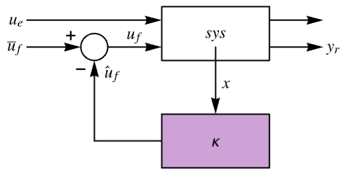
 - The inputs u of sys consist of feedback inputs uf and possibly other inputs ue.
- The outputs y of sys consist of regulated outputs yr and possibly other outputs.
- The system specification sspec is the system sys together with the uf and yr specifications.
- LQOutputRegulatorGains minimizes a quadratic cost function with weights q, r and p of the regulated outputs yr and feedback inputs uf of a linear system sys:
-

continuous-time system 
discrete-time system - LQ design works for linear systems as specified by StateSpaceModel:
-

continuous-time system 
discrete-time system - The resulting feedback gain matrix is then computed as
![kappa=TemplateBox[{{r, _, 1}}, Inverse].x_1](Files/LQOutputRegulatorGains.en/8.png "kappa=TemplateBox[{{r, _, 1}}, Inverse].x_1") :
: -


continuous-time system 

discrete-time system - The matrix xr is the solution of the Riccati equation:
-
![a.x_r+x_r.a-x_1.TemplateBox[{{r, _, 1}}, Inverse].x_1+c_r.q.c_r=0](Files/LQOutputRegulatorGains.en/13.png "a.x_r+x_r.a-x_1.TemplateBox[{{r, _, 1}}, Inverse].x_1+c_r.q.c_r=0")
continuous-time algebraic Riccati equation ![a.x_r.a-x_r-x_1.TemplateBox[{{r, _, 1}}, Inverse].x_1+c_r.q.c_r=0](Files/LQOutputRegulatorGains.en/14.png "a.x_r.a-x_r-x_1.TemplateBox[{{r, _, 1}}, Inverse].x_1+c_r.q.c_r=0")
discrete-time algebraic Riccati equation - The submatrices bf, cr and drf correspond to the feedback inputs uf and regulated outputs yr.
- The weights wts can have the following forms:
-
{q,r} cost function with no cross-coupling {q,r,p} cost function with cross-coupling matrix p - The system specification sspec can have the following forms:
-
StateSpaceModel[…] linear control input and linear state AffineStateSpaceModel[…] linear control input and nonlinear state NonlinearStateSpaceModel[…] nonlinear control input and nonlinear state SystemModel[…] general system model <…> detailed system specification given as an Association - The detailed system specification can have the following keys:
-
"InputModel" sys any one of the models "FeedbackInputs" All the feedback inputs uf "RegulatedOutputs" All the regulated outputs yr - The inputs and outputs can have the following forms:
-
{num1,…,numn} numbered inputs or outputs numi used by StateSpaceModel, AffineStateSpaceModel and NonlinearStateSpaceModel {name1,…,namen} named inputs or outputs namei used by SystemModel All uses all inputs or outputs - For nonlinear systems such as AffineStateSpaceModel, NonlinearStateSpaceModel and SystemModel, the system will be linearized around its stored operating point.
- LQOutputRegulatorGains[…,"Data"] returns a SystemsModelControllerData object cd that can be used to extract additional properties using the form cd["prop"].
- LQOutputRegulatorGains[…,"prop"] can be used to directly give the value of cd["prop"].
- Possible values for properties "prop" include:
-
"ClosedLoopPoles" poles of the linearized "ClosedLoopSystem" "ClosedLoopSystem" system csys with ue and  as input and y as output
{"ClosedLoopSystem", cspec} detailed control over the form of the closed-loop system "ControllerModel" model cm with  and x as input and uf as output
 "Design" type of controller design "DesignModel" model used for the design "FeedbackGains" gain matrix κ or its equivalent "FeedbackGainsModel" model gm with x as input and  as output
"FeedbackInputs" inputs uf of sys used for feedback "InputModel" input model sys "InputCount" number of inputs u of sys "OpenLoopPoles" poles of "DesignModel" "OutputCount" number of outputs y of sys "RegulatedOutputs" outputs yr of sys that are regulated "SamplingPeriod" sampling period of sys "StateCount" number of states x of sys - Possible keys for cspec include:
-
"InputModel" input model in csys "Merge" whether to merge csys "ModelName" name of csys

The diagram of the feedback gains model gm, controller model cm and closed-loop system csys.
[image]Examples
open all close allBasic Examples (2)
A set of optimal output-weighted state feedback gains for a continuous-time system:
LQOutputRegulatorGains[StateSpaceModel[{{{0, 1, 0}, {0, -0.01, 0.3}, {0, -0.003, -10}}, {{0, 0}, {0, -1}, {0.1, 0}},
  {{1, 0, 0}, {0, 1, 0}}, {{1, 0}, {0, 1}}}, SamplingPeriod -> None, SystemsModelLabels -> None], {(|   |   |
| - | - |
| 1 | 0 |
| 0 | 1 |), (|     |     |
| --- | --- |
| 0.1 | 0   |
| 0   | 0.1 |)}]//MatrixForm
LQ output regulator gains for a discrete-time system:
LQOutputRegulatorGains[StateSpaceModel[{{{-0.05156, -0.05877}, {0.01503, -0.005887}}, {{0}, {-0.03384}},
  {{1.1, -0.5}, {-0.7, 1}}, {{0.1}, {0.2}}}, SamplingPeriod -> 0.1, SystemsModelLabels -> None], {(|    |     |
| -- | --- |
| 10 | 0   |
| 0  | 0.1 |), {{1}}}]
Scope (27)
Basic Uses (8)
Compute the state feedback gain of a system with equal weighting for the output and input:
ssm = StateSpaceModel[{{{-10}}, {{1}}, {{1}}, {{1}}}, SamplingPeriod -> None, SystemsModelLabels -> None];κ = LQOutputRegulatorGains[ssm, {{{1}}, {{1}}}]SystemsModelStateFeedbackConnect[ssm, κ]//SimplifyCompute the gain for an unstable system:
ssm = StateSpaceModel[{{{10}}, {{1}}, {{1}}, {{1}}}, SamplingPeriod -> None, SystemsModelLabels -> None];κ = LQOutputRegulatorGains[ssm, {{{1}}, {{1}}}]The gain stabilizes the unstable system:
SystemsModelStateFeedbackConnect[ssm, κ]//SimplifyCompute the state feedback gains for a multiple-output system:
ssm = StateSpaceModel[{{{0, 0, -0.1}, {1., 0., -1.08}, {0., 1., -0.9}}, {{1}, {1}, {0}},
{{0, 1, 1}, {0, 0, 1}}, {{0}, {0}}}, SamplingPeriod -> None, SystemsModelLabels -> None];κ = LQOutputRegulatorGains[ssm, {(| | |
| - | - |
| 1 | 0 |
| 0 | 2 |), (0.5)}]The dimensions of the result correspond to the number of inputs and the system's order:
Dimensions[κ]{SystemsModelDimensions[ssm][[1]], SystemsModelOrder[ssm]}Compute the gains for a system with 3 outputs and 2 inputs:
ssm = StateSpaceModel[{{{0, 0, -0.1, 0}, {1., 0., -1.08, 0.1}, {0., 1., -0.9, -1}, {0, 1, 0, 0}},
  {{1, 0}, {0, 1}, {0, 0}, {0, 0}}, {{1, 0, 0, 1}, {0, 1, 0, 1}, {0, 0, 1, 1}},
{{0, 0}, {0, 0}, {0, 0}}}, SamplingPeriod -> None, SystemsModelLabels -> None];MatrixForm[κ1 = LQOutputRegulatorGains[ssm, {(| | | |
| - | - | -- |
| 1 | 0 | 0 |
| 0 | 1 | 0 |
| 0 | 0 | 10 |), (| | |
| - | - |
| 1 | 0 |
| 0 | 5 |)}]]Reverse the weights of the feedback inputs:
MatrixForm[κ2 = LQOutputRegulatorGains[ssm, {(| | | |
| - | - | -- |
| 1 | 0 | 0 |
| 0 | 1 | 0 |
| 0 | 0 | 10 |), (| | |
| - | - |
| 5 | 0 |
| 0 | 1 |)}]]Typically, the feedback input with the bigger weight has the smaller norm:
Norm /@ κ1
Norm /@ κ2
Compute the gains when the cost function contains cross-coupling of the outputs and feedback inputs:
ssm = StateSpaceModel[{{{0, 0, -0.1}, {1., 0., -1.08}, {0., 1., -0.9}}, {{1, 1}, {1, 0}, {0, 0}},
{{1, 0, 1}}, {{0, 0}}}, SamplingPeriod -> None, SystemsModelLabels -> None];LQOutputRegulatorGains[ssm, {(1), (| | |
| - | - |
| 1 | 0 |
| 0 | 1 |), (0.1 0.1)}]//MatrixFormChoose the feedback outputs for multiple-output systems:
ssm = StateSpaceModel[{{{0, 1., 0.}, {0, 0., 1.}, {-0.1, -1.08, -0.9}}, {{0}, {0}, {1}},
{{1, 1, 0}, {1, 0, 0}}, {{0}, {0}}}, SamplingPeriod -> None, SystemsModelLabels -> None];wts = {(1), (5)};LQOutputRegulatorGains[<|"InputModel" -> ssm, "RegulatedOutputs" -> 1|>, wts]LQOutputRegulatorGains[<|"InputModel" -> ssm, "RegulatedOutputs" -> 2|>, wts]Choose the feedback inputs for multiple-input systems:
ssm = StateSpaceModel[{{{0, 0, -0.1}, {1., 0., -1.08}, {0., 1., -0.9}}, {{1, 1}, {1, 0}, {0, 0}},
{{1, 0, 1}}, {{0, 0}}}, SamplingPeriod -> None, SystemsModelLabels -> None];wts = {(1), (5)};LQOutputRegulatorGains[<|"InputModel" -> ssm, "FeedbackInputs" -> 1|>, wts]LQOutputRegulatorGains[<|"InputModel" -> ssm, "FeedbackInputs" -> 2|>, wts]Compute the gains for a nonlinear system:
nssm = NonlinearStateSpaceModel[{{u + x + x^2},
  {-1 + x}}, {{x, 1}}, {{u, -2}}, {Automatic}, Automatic,
 SamplingPeriod -> None];
The controller is returned as a vector and takes operating points into consideration:
LQOutputRegulatorGains[nssm, {{{10}}, {{1}}}]The controller for the approximate linear system:
LQOutputRegulatorGains[StateSpaceModel[nssm], {{{10}}, {{1}}}]Plant Models (6)
Continuous-time StateSpaceModel:
LQOutputRegulatorGains[StateSpaceModel[{{{0, 1.}, {-1, -1.6}}, {{0}, {1}}, {{1, 1}, {0, 1}}, {{0}, {0}}},
SamplingPeriod -> None, SystemsModelLabels -> None], {(| | |
| - | - |
| 1 | 0 |
| 0 | 1 |), (1)}]Discrete-time StateSpaceModel:
LQOutputRegulatorGains[StateSpaceModel[{{{0, 1.}, {0.020000000000000004, 0.1}}, {{0}, {1}}, {{1, 1}, {0, 1}}, {{0}, {0}}},
SamplingPeriod -> τ, SystemsModelLabels -> None], {(| | |
| - | - |
| 1 | 0 |
| 0 | 1 |), (1)}]Descriptor StateSpaceModel:
LQOutputRegulatorGains[StateSpaceModel[{{{-6, -4}, {-6, -5}}, {{1}, {1}}, {{1, 1}, {0, 1}}, {{0}, {0}}, {{1, 1}, {0, 1}}},
{{x1[t], 0}, {x2[t], 0}},
{{u[t], 0}}, Automatic, t, SamplingPeriod -> None,
SystemsModelLabels -> None], {(| | |
| - | - |
| 1 | 0 |
| 0 | 1 |), (1.0)}]LQOutputRegulatorGains[AffineStateSpaceModel[{{Sin[Subscript[x, 1]] + Subscript[x, 2],
-Subscript[x, 1] - Subscript[x, 2]},
{{Subscript[x, 1]}, {1}},
{Subscript[x, 1] - Subscript[x, 2], Subscript[x, 2]},
{{0}, {0}}}, {Subscript[x, 1], Subscript[x, 2]}, {{u, 0}},
{Automatic, Automatic}, Automatic, SamplingPeriod -> None], {(| | |
| - | - |
| 1 | 0 |
| 0 | 1 |), (1.0)}]LQOutputRegulatorGains[NonlinearStateSpaceModel[
{{Subscript[x, 2] + Subscript[x, 1]*Subscript[x, 2],
u + Subscript[x, 1]},
{Subscript[x, 1] - Subscript[x, 2], Subscript[x, 2]}},
{Subscript[x, 1], Subscript[x, 2]}, {u},
{Automatic, Automatic}, Automatic, SamplingPeriod -> None], {(| | |
| - | - |
| 1 | 0 |
| 0 | 1 |), (1.0)}]sm = CreateSystemModel[{x''[t] + x'[t] + x[t] == u[t], y1[t] == x[t], y2[t] == x'[t]}, t, {"u"∈"Modelica.Blocks.Interfaces.RealInput", {"y1", "y2"}∈"Modelica.Blocks.Interfaces.RealOutput"}];LQOutputRegulatorGains[sm, {(| | |
| - | - |
| 1 | 0 |
| 0 | 1 |), (1)}]Properties (10)
LQOutputRegulatorGains returns the feedback gains by default:
ssm = StateSpaceModel[{{{0, 1}, {-1, -2}}, {{0}, {1}}, {{1, 1}}, {{0}}}, SamplingPeriod -> None,
SystemsModelLabels -> None];wts = {(1.0), (1.0)};LQOutputRegulatorGains[ssm, wts]% == LQOutputRegulatorGains[ssm, wts, "FeedbackGains"]In general, the feedback is affine in the states:
κ = LQOutputRegulatorGains[NonlinearStateSpaceModel[
{{-Subscript[x, 1] + u*Subscript[x, 1] +
Subscript[x, 2]/E^Subscript[x, 1],
E^Subscript[x, 2] - Subscript[x, 1]},
{u + Subscript[x, 1], Subscript[x, 2]}},
{{Subscript[x, 1], 1}, {Subscript[x, 2], 0}}, {{u, 1.}},
{Automatic, Automatic}, Automatic, SamplingPeriod -> None], {(| | |
| - | - |
| 1 | 0 |
| 0 | 1 |), (1)}]It is of the form κ0+κ1.x, where κ0 and κ1 are constants:
{κ0, κ1} = {κ /. {Subscript[x, _] -> 0}, D[κ, {{Subscript[x, 1], Subscript[x, 2]}}]}The systems model of the feedback gains:
LQOutputRegulatorGains[StateSpaceModel[{{{0, 1}, {-1, -2}}, {{0}, {1}}, {{1, 1}}, {{0}}}, SamplingPeriod -> None,
SystemsModelLabels -> None], {(1.0), (1.0)}, "FeedbackGainsModel"]An affine systems model of the feedback gains:
LQOutputRegulatorGains[NonlinearStateSpaceModel[{{Subscript[x, 2], -2/3 + u -
Subscript[x, 1]/3 - Subscript[x, 2]/2},
{Subscript[x, 1] + Subscript[x, 2]}},
{{Subscript[x, 1], 1}, {Subscript[x, 2], 0}}, {{u, 1.}},
{Automatic}, Automatic, SamplingPeriod -> None], {(1.0), (1.0)}, "FeedbackGainsModel"]//ChopLQOutputRegulatorGains[StateSpaceModel[{{{0., 1.}, {-0.05, -0.9}}, {{0}, {1}}, {{1, 1}, {0, 1}}, {{0}, {0}}},
{Subscript[x, 1], Subscript[x, 2]}, {{f, 0}},
SamplingPeriod -> None, SystemsModelLabels -> None], {(| | |
| - | - |
| 1 | 0 |
| 0 | 1 |), (1)}, "ClosedLoopSystem"]The poles of the linearized closed-loop system:
assm = AffineStateSpaceModel[{{Subscript[x, 2], -0.05*Subscript[x, 1] -
0.9*Subscript[x, 2]^2}, {{0}, {1}},
{Subscript[x, 1] + Subscript[x, 2], Subscript[x, 2]},
{{0}, {0}}}, {Subscript[x, 1], Subscript[x, 2]}, {{f, 0}},
{Automatic, Automatic}, Automatic, SamplingPeriod -> None];
wts = {(| | |
| - | - |
| 1 | 0 |
| 0 | 1 |), (1)};LQOutputRegulatorGains[assm, wts, "ClosedLoopPoles"]The model used to compute the feedback gains:
assm = AffineStateSpaceModel[{{Subscript[x, 2], -0.05*Subscript[x, 1] -
0.9*Subscript[x, 2]^2}, {{0}, {1}},
{Subscript[x, 1] + Subscript[x, 2], Subscript[x, 2]},
{{0}, {0}}}, {Subscript[x, 1], Subscript[x, 2]}, {{f, 0}},
{Automatic, Automatic}, Automatic, SamplingPeriod -> None];
wts = {(| | |
| - | - |
| 1 | 0 |
| 0 | 1 |), (1)};dmodel = LQOutputRegulatorGains[assm, wts, "DesignModel"]The gains of the design model and input model:
LQOutputRegulatorGains[dmodel, wts]
LQOutputRegulatorGains[assm, wts]LQOutputRegulatorGains[AffineStateSpaceModel[{{Subscript[x, 2], -0.05*Subscript[x, 1] -
0.9*Subscript[x, 2]^2}, {{0}, {1}},
{Subscript[x, 1] + Subscript[x, 2], Subscript[x, 2]},
{{0}, {0}}}, {Subscript[x, 1], Subscript[x, 2]}, {{f, 0}},
{Automatic, Automatic}, Automatic, SamplingPeriod -> None], {(| | |
| - | - |
| 1 | 0 |
| 0 | 1 |), (1)}, "Design"]Properties related to the input model:
Dataset[Table[{prop, LQOutputRegulatorGains[IconizedObject[«sys»], IconizedObject[«wts»], prop]}, {prop, IconizedObject[«props»]}]]Get the controller data object:
𝒸𝒹 = LQOutputRegulatorGains[IconizedObject[«sys»], IconizedObject[«wts»], "Data"]The list of available properties:
𝒸𝒹["Properties"]The value of a specific property:
𝒸𝒹["ClosedLoopPoles"]Closed-Loop System (3)
Assemble the closed-loop system for a nonlinear plant model:
assm = AffineStateSpaceModel[{{Subscript[x, 1] - Subscript[x, 1]^2 -
    Subscript[x, 2], Subscript[x, 1]}, {{0}, {1}},
  {Subscript[x, 1] + Subscript[x, 2]}, {{0}}},
 {Subscript[x, 1], Subscript[x, 2]}, {u}, {Automatic},
Automatic, SamplingPeriod -> None];csys1 = LQOutputRegulatorGains[assm, {(1.0), (1.0)}, "ClosedLoopSystem"]The closed-loop system with a linearized model:
csys2 = LQRegulatorGains[assm, {(| | |
| - | - |
| 1 | 0 |
| 0 | 1 |), (1.0)}, {"ClosedLoopSystem", <|"InputModel" -> AffineStateSpaceModel[{{Subscript[x, 1] - Subscript[x, 2],
Subscript[x, 1]}, {{0}, {1}},
{Subscript[x, 1] + Subscript[x, 2]}, {{0}}},
{Subscript[x, 1], Subscript[x, 2]}, {u}, {Automatic},
Automatic, SamplingPeriod -> None]|>}]Compare the response of the two systems:
Table[OutputResponse[{sys, {0.5, 1}}, 0, {t, 0, 7}], {sys, {csys1, csys2}}];
Plot[%, {t, 0, 7}, PlotLegends -> {"Nonlinear", "Linear"}, PlotRange -> All]
Assemble the merged closed-loop of a plant with one disturbance and one feedback input:
sys = <|"InputModel" -> StateSpaceModel[{{{0., 1.}, {-0.05, -0.9}}, {{0, 0}, {1, 1}}, {{1, 1}}, {{0, 0}}},
 {Subscript[x, 1], Subscript[x, 2]},
 {{d, 0}, {f, 0}}, SamplingPeriod -> None,
 SystemsModelLabels -> {{Subscript[u, e],
Subscript[u, f]}}], "FeedbackInputs" -> 2|>;wts = {(1.0), (1.0)};LQOutputRegulatorGains[sys, wts, "ClosedLoopSystem"]The unmerged closed-loop system:
LQOutputRegulatorGains[sys, wts, {"ClosedLoopSystem", <|"Merge" -> False|>}]When merged, it gives the same result as before:
SystemsModelMerge[%]Explicitly specify the merged closed-loop system:
LQOutputRegulatorGains[sys, wts, {"ClosedLoopSystem", <|"Merge" -> True|>}]Create a closed-loop system with a desired name:
sm = CreateSystemModel["MassSpringDamper", {m x''[t] + c x'[t] + k x[t] == u[t], y1[t] == x[t], y2[t] == x'[t]}, t, {"u"∈"Modelica.Blocks.Interfaces.RealInput", {"y1", "y2"}∈"Modelica.Blocks.Interfaces.RealOutput"}, <|"ParameterValues" -> {m -> 10, c -> 10^2, k -> 10^3}|>];csysName = "MassSpringDamperWithStateFeedback";csys = LQOutputRegulatorGains[sm, {(| | |
| - | - |
| 1 | 0 |
| 0 | 1 |), (1)}, {"ClosedLoopSystem", <|"ModelName" -> csysName|>}]The closed-loop system has the specified name:
csys["ModelName"]The name can be directly used to specify the closed-loop model in other functions:
SystemModelSimulate[csysName, {"y1", "y2"}, 2, <|"Inputs" -> {"u" -> UnitStep}|>]SystemModelPlot[%, All, PlotRange -> All]Applications (2)
Construct an output-weighted state-feedback gain matrix for an aircraft model:
aircraftM = StateSpaceModel[{{{0.4158, 1.025, -0.00267, -0.00011106, -0.08021, 0},
   {-5.5, -0.8302, -0.06549, -0.0039, -5.115, 0.809}, {0, 0, 0, 1, 0, 0},
   {-1040, 78.35, -34.83, -0.6214, -865.6, -631}, {0, 0, 0, 0, -75, 0}, {0, 0, 0, 0, 0, -100}},
  {{0, 0}, {0, 0}, {0, 0}, {0, 0}, {75, 0}, {0, 100}}, {{1, 0, 0, 0, 2, 0}, {0, 1, 0, 0, 0, 0}},
{{0, 0}, {0, 0}}}, SamplingPeriod -> None, SystemsModelLabels -> None];k = LQOutputRegulatorGains[aircraftM, {(| | |
| ------ | - |
| 0.0001 | 0 |
| 0 | 1 |), (| | |
| - | - |
| 1 | 0 |
| 0 | 1 |)}]Plot the closed-loop output response:
aircraftMCL = SystemsModelStateFeedbackConnect[aircraftM, k];or = OutputResponse[{aircraftMCL, {0, 0.1, 0, 0, 0, 0}}, {0, 0}, {t, 0, 6}];Plot[or, {t, 0, 6}, PlotRange -> All, PlotLegends -> {Subscript[y, 1], Subscript[y, 2]}]fb = -k.StateResponse[{aircraftMCL, {0, 0.1, 0, 0, 0, 0}}, {0, 0}, {t, 6}];Plot[fb, {t, 0, 6}, PlotRange -> All, PlotLegends -> {Subscript[u, 1], Subscript[u, 2]}]A two-loop circuit modeled as a descriptor system:
circuit = StateSpaceModel[{{{0, 0, 0, 1}, {0, 0, 1, 0}, {-1, 1, 0, 0}, {1, 0, 10, 10}},
  {{0}, {0}, {0}, {-1}}, {{0, 0.1, 0, 0}}, {{0}}, {{0.1, 0, 0, 0}, {0, 0.2, 0, 0},
   {0, 0, -0.01, 0}, {0, 0, 0, 0}}}, Automatic, SamplingPeriod -> None, SystemsModelLabels -> None];
The circuit has a large magnitude response at certain frequencies:
openloopresponse = OutputResponse[circuit, Sin[6 2 Pi t], {t, 0, 1}];
Plot[openloopresponse, {t, 0, 1}, PlotRange -> All]
Find an optimal closed-loop system for unity cost matrices:
k = LQOutputRegulatorGains[circuit, {{{1}}, {{1}}}];
clssm = SystemsModelStateFeedbackConnect[circuit, k]
The closed-loop response is attenuated:
closedloopresponse = OutputResponse[clssm, Sin[6 2 Pi t], {t, 0, 1}];
Plot[closedloopresponse, {t, 0, 1}, PlotRange -> All]
Properties & Relations (3)
Equivalent output regulator gains can be computed using LQRegulatorGains:
{a, b, c, d} = {(| | | |
| -- | -- | -- |
| -2 | 0 | 1 |
| 0 | -1 | 0 |
| -3 | -4 | -2 |), (| | |
| - | - |
| 0 | 1 |
| 0 | 0 |
| 1 | 0 |), (| | | |
| - | - | - |
| 1 | 0 | 0 |
| 0 | 1 | 0 |), (| | |
| - | - |
| 1 | 0 |
| 0 | 2 |)};{q, r, p} = {(| | |
| --- | --- |
| 100 | 0. |
| 0 | 0.1 |), (| | |
| -- | - |
| 10 | 0 |
| 0 | 1 |), (| | |
| - | - |
| 1 | 0 |
| 0 | 1 |)};ssm = StateSpaceModel[{a, b, c, d}];LQRegulatorGains[ssm, {c.q.c, r + d.q.d + d.p + p.d, c.q.d + c.p}]LQOutputRegulatorGains gives the same result:
LQOutputRegulatorGains[ssm, {q, r, p}] - %Compute the LQ output regulator gains by solving the underlying Riccati equation:
{a, b, c, d} = {(| | | | | |
| - | -------- | ------- | - | ------- |
| 0 | -0.01156 | -0.1711 | 0 | 0 |
| 0 | -0.1419 | 0.1711 | 0 | 0 |
| 0 | -0.00875 | -1.102 | 0 | 0 |
| 0 | -0.00128 | -0.1489 | 0 | 0.00013 |
| 0 | 0.0605 | 0.1489 | 0 | -0.0591 |), (| | | |
| ----- | ------- | ------- |
| 0 | -0.143 | 0 |
| 0 | 0 | 0 |
| 0.392 | 0 | 0 |
| 0 | 0.108 | -0.0592 |
| 0 | -0.0486 | 0 |), (| | | | | |
| - | - | - | - | - |
| 1 | 0 | 0 | 0 | 0 |
| 0 | 0 | 0 | 1 | 0 |
| 0 | 0 | 0 | 0 | 1 |), (| | | |
| - | - | - |
| 0 | 1 | 0 |
| 1 | 0 | 0 |
| 0 | 0 | 1 |)};{q, r, p} = {(| | | |
| ---- | --- | -- |
| 1000 | 0 | 0 |
| 0 | 100 | 0 |
| 0 | 0 | 10 |), (| | | |
| - | - | -- |
| 1 | 0 | 0 |
| 0 | 1 | 0 |
| 0 | 0 | 10 |), (| | | |
| --- | - | - |
| 100 | 0 | 0 |
| 0 | 1 | 0 |
| 0 | 0 | 1 |)};With[{q = c.q.c, r = r + d.q.d + d.p + p.d, p = c.q.d + c.p}, Inverse[r].(b.RiccatiSolve[{a, b}, {q, r, p}] + p)]LQOutputRegulatorGains gives the same result:
LQOutputRegulatorGains[StateSpaceModel[{a, b, c, d}], {q, r, p}] - %//ChopCompute the gains for a discrete-time system using DiscreteRiccatiSolve:
{a, b, c, d} = {(| | | | | |
| - | -------- | ------- | - | ------- |
| 1 | -0.01866 | -0.134 | 0 | 0 |
| 0 | 0.7516 | 0.1144 | 0 | 0 |
| 0 | -0.0059 | 0.1097 | 0 | 0 |
| 0 | -0.0009 | -0.1203 | 1 | 0.00025 |
| 0 | 0.0978 | 0.1206 | 0 | 0.8885 |), (| | | |
| ------- | ------- | ------- |
| -0.0732 | -0.286 | 0 |
| 0.0652 | 0 | 0 |
| 0.3162 | 0 | 0 |
| -0.0632 | 0.216 | -0.1184 |
| 0.0634 | -0.0917 | 0 |), (| | | | | |
| - | - | - | - | - |
| 1 | 0 | 0 | 0 | 0 |
| 0 | 0 | 0 | 1 | 0 |
| 0 | 0 | 0 | 0 | 1 |), (| | | |
| - | - | - |
| 0 | 1 | 0 |
| 1 | 0 | 0 |
| 0 | 0 | 1 |)};{q, r, p} = {(| | | |
| ---- | --- | -- |
| 1000 | 0 | 0 |
| 0 | 100 | 0 |
| 0 | 0 | 10 |), (| | | |
| - | - | -- |
| 1 | 0 | 0 |
| 0 | 1 | 0 |
| 0 | 0 | 10 |), (| | | |
| --- | - | - |
| 100 | 0 | 0 |
| 0 | 1 | 0 |
| 0 | 0 | 1 |)};With[{q = c.q.c, r = r + d.q.d + d.p + p.d, p = c.q.d + c.p}, With[{x = DiscreteRiccatiSolve[{a, b}, {q, r, p}]}, Inverse[b.x.b + r].(b.x.a + p)]]LQOutputRegulatorGains gives the same result:
LQOutputRegulatorGains[StateSpaceModel[{a, b, c, d}, SamplingPeriod -> τ], {q, r, p}] - %//ChopText
Wolfram Research (2010), LQOutputRegulatorGains, Wolfram Language function, https://reference.wolfram.com/language/ref/LQOutputRegulatorGains.html (updated 2021).
CMS
Wolfram Language. 2010. "LQOutputRegulatorGains." Wolfram Language & System Documentation Center. Wolfram Research. Last Modified 2021. https://reference.wolfram.com/language/ref/LQOutputRegulatorGains.html.
APA
Wolfram Language. (2010). LQOutputRegulatorGains. Wolfram Language & System Documentation Center. Retrieved from https://reference.wolfram.com/language/ref/LQOutputRegulatorGains.html