RiccatiSolve[{a,b},{q,r}]
gives the matrix ![]() that is the stabilizing solution of the continuous algebraic Riccati equation
that is the stabilizing solution of the continuous algebraic Riccati equation ![]() .
.
RiccatiSolve[{a,b},{q,r,p}]
solves the equation ![]() .
.


RiccatiSolve
RiccatiSolve[{a,b},{q,r}]
gives the matrix ![]() that is the stabilizing solution of the continuous algebraic Riccati equation
that is the stabilizing solution of the continuous algebraic Riccati equation ![]() .
.
RiccatiSolve[{a,b},{q,r,p}]
solves the equation ![]() .
.
Details and Options
- In
![TemplateBox[{a}, ConjugateTranspose].x+x.a-x.b.TemplateBox[{r}, Inverse].TemplateBox[{b}, ConjugateTranspose].x+q=0](Files/RiccatiSolve.en/4.png "TemplateBox[{a}, ConjugateTranspose].x+x.a-x.b.TemplateBox[{r}, Inverse].TemplateBox[{b}, ConjugateTranspose].x+q=0") ,
,  denotes the conjugate transpose.
 - The equation
![TemplateBox[{a}, ConjugateTranspose].x+x.a-x.b.TemplateBox[{r}, Inverse].TemplateBox[{b}, ConjugateTranspose].x+q=0](Files/RiccatiSolve.en/6.png "TemplateBox[{a}, ConjugateTranspose].x+x.a-x.b.TemplateBox[{r}, Inverse].TemplateBox[{b}, ConjugateTranspose].x+q=0") has a unique, symmetric, positive semidefinite solution
has a unique, symmetric, positive semidefinite solution  if
if  is stabilizable,
  is detectable,
  , and
, and  . Consequently, all eigenvalues of the matrix
  are negative and the solution is stabilizing.
 - The solution is positive definite when
 is controllable and
  is observable.
 - RiccatiSolve supports a Method option, with the following possible settings:
-
Automatic automatically determined method "Eigensystem" based on eigen decomposition "GeneralizedEigensystem" based on generalized eigen decomposition "GeneralizedSchur" based on generalized Schur decomposition "InverseFree" a variant of "GeneralizedSchur" "MatrixSign" iterative method using the matrix sign function "Newton" iterative Newton method "Schur" based on Schur decomposition - All methods apply to approximate numeric matrices. "Eigensystem" also applies to exact matrices.
Examples
open all close allBasic Examples (1)
Solve a continuous algebraic Riccati equation:
{a, b, q, r} = {(| | |
| -- | - |
| -3 | 2 |
| 1 | 1 |), (| |
| - |
| 0 |
| 1 |), (| | |
| --- | --- |
| 1. | -1. |
| -1. | 1. |), (3)};x = RiccatiSolve[{a, b}, {q, r}]Transpose[a].x + x.a - x.b.Inverse[r].Transpose[b].x + q//ChopScope (3)
Solve a continuous Riccati equation:
RiccatiSolve[{(|    |    |    |
| -- | -- | -- |
| -1 | 0  | 0  |
| 0  | -4 | 0  |
| 0  | 0  | -6 |), (|    |
| -- |
| 3  |
| 1  |
| -1 |)}, {(|   |   |   |
| - | - | - |
| 4 | 2 | 0 |
| 2 | 4 | 0 |
| 0 | 0 | 1 |), {{1.}}}]//MatrixForm
Solve a Riccati equation with state-control coupling:
RiccatiSolve[{(|   |        |     |
| - | ------ | --- |
| 0 | 1      | 0   |
| 0 | -0.01  | 0.3 |
| 0 | -0.003 | -10 |), (|     |    |
| --- | -- |
| 0   | 0  |
| 0   | -1 |
| 0.1 | 0  |)}, {(|   |   |   |
| - | - | - |
| 1 | 0 | 0 |
| 0 | 1 | 0 |
| 0 | 0 | 1 |), (|   |   |
| - | - |
| 1 | 0 |
| 0 | 1 |), (|      |     |
| ---- | --- |
| 0.1  | 0   |
| -0.2 | 0   |
| 0.15 | 0.2 |)}]
Solve the Riccati equation by extracting appropriate matrices from a state-space model object:
ssm = StateSpaceModel[{{{0.4245, 0.1137}, {-0.4145, -0.0987}}, {{9.764, 0}, {-6.32, -3.455}}},
SamplingPeriod -> None, SystemsModelLabels -> None];{q, r} = {(| | |
| ---- | ---- |
| 84.4 | 0 |
| 0 | 6.16 |), (| | |
| ----- | ----- |
| 10^-3 | 0 |
| 0 | 10^-3 |)};RiccatiSolve[Normal[ssm][[1 ;; 2]], {q, r}]Options (7)
Method (7)
Automatic and "Eigensystem" methods can be used for exact systems:
x1 = RiccatiSolve[{(| | |
| - | - |
| 1 | 0 |
| 0 | 1 |), (| | |
| - | - |
| 1 | 0 |
| 0 | 1 |)}, {(| | |
| - | - |
| 1 | 0 |
| 0 | 1 |), (| | |
| - | - |
| 1 | 0 |
| 0 | 1 |)}, Method -> Automatic]x2 = RiccatiSolve[{(| | |
| - | - |
| 1 | 0 |
| 0 | 1 |), (| | |
| - | - |
| 1 | 0 |
| 0 | 1 |)}, {(| | |
| - | - |
| 1 | 0 |
| 0 | 1 |), (| | |
| - | - |
| 1 | 0 |
| 0 | 1 |)}, Method -> "Eigensystem"]x1 == x2As well as for inexact systems:
x1 = RiccatiSolve[N@{(| | |
| - | - |
| 1 | 0 |
| 0 | 1 |), (| | |
| - | - |
| 1 | 0 |
| 0 | 1 |)}, {(| | |
| - | - |
| 1 | 0 |
| 0 | 1 |), (| | |
| - | - |
| 1 | 0 |
| 0 | 1 |)}, Method -> Automatic]x2 = RiccatiSolve[N@{(| | |
| - | - |
| 1 | 0 |
| 0 | 1 |), (| | |
| - | - |
| 1 | 0 |
| 0 | 1 |)}, {(| | |
| - | - |
| 1 | 0 |
| 0 | 1 |), (| | |
| - | - |
| 1 | 0 |
| 0 | 1 |)}, Method -> "Eigensystem"]x1 == x2"Schur" method can be used for inexact systems:
RiccatiSolve[{N@(| | |
| - | - |
| 1 | 0 |
| 0 | 1 |), (| | |
| - | - |
| 1 | 0 |
| 0 | 1 |)}, {(| | |
| - | - |
| 1 | 0 |
| 0 | 1 |), (| | |
| - | - |
| 1 | 0 |
| 0 | 1 |)}, Method -> "Schur"]"Newton" applies to inexact systems and may be more accurate than Automatic:
a = SparseArray[{{1, 1} -> 0.8, {1, 5} -> -0.8, {2, 1} -> 0.8, {2, 2} -> 1, {3, 3} -> -0.1, {2, 5} -> -0.5, {5, 1} -> 0.25}];
b = Transpose[{{1, 0, 0, 1, 0}}];
r = {{1}};
q = IdentityMatrix[5];
Compute the solution and absolute error:
x1 = RiccatiSolve[{a, b}, {q, r}, Method -> "Newton"];Norm[a^.x1 + x1.a - x1.b.Inverse[r].b^.x1 + q]Compare to the default method:
x2 = RiccatiSolve[{a, b}, {q, r}];Norm[a^.x2 + x2.a - x2.b.Inverse[r].b^.x2 + q]"Newton" takes suboptions "StartingMatrix", "MaxIterations", and "Tolerance":
x3 = RiccatiSolve[{a, b}, {q, r}, Method -> {"Newton", "StartingMatrix" -> x2, "Tolerance" -> 10^-13, "MaxIterations" -> 20}];Norm[a^.x3 + x3.a - x3.b.Inverse[r].b^.x3 + q]The "Newton" method may not converge even if a stabilizing solution exists:
a = ConstantArray[0., {5, 5}];
r = b = q = IdentityMatrix[5];
RiccatiSolve[{a, b}, {q, r}, Method -> "Newton"];
Compare with the Automatic method:
x = RiccatiSolve[{a, b}, {q, r}]"MatrixSign" is typically used as an initial approximation for the "Newton" method:
{a, b} = {{{-0.1, 0}, {0, -0.02}}, {{0.1, 0}, {0.001, 0.01}}};
{q, r} = {{{100, 1000}, {1000, 10^4}}, {{1. + 10^-6, 1.}, {1., 1.}}};xinit = RiccatiSolve[{a, b}, {q, r}, Method -> "MatrixSign"];Use xinit to initialize the "Newton" method:
x = RiccatiSolve[{a, b}, {q, r}, Method -> {"Newton", "StartingMatrix" -> xinit, "Tolerance" -> 10^-10, "MaxIterations" -> 10}];Map[Norm[a^.# + #.a - #.b.Inverse[r].b^.# + q]&, {xinit, x}]"MatrixSign" takes suboptions "MaxIterations" and "Tolerance":
x3 = RiccatiSolve[{a, b}, {q, r}, Method -> {"MatrixSign", "Tolerance" -> 10^-10, "MaxIterations" -> 10}];Norm[a^.x3 + x3.a - x3.b.Inverse[r].b^.x3 + q]"GeneralizedSchur" and "GeneralizedEigensystem" applies when a is singular:
a = SparseArray[{{1, 1} -> 0.8, {1, 5} -> -0.8, {2, 1} -> 0.8, {2, 5} -> -0.5, {2, 2} -> 1, {3, 3} -> -0.1, {5, 1} -> 0.25}];
b = Transpose[{{1, 0, 0, 1, 0}}];
r = {{1}};
q = IdentityMatrix[5];Det[a]These two methods work for a singular a:
x1 = RiccatiSolve[{a, b}, {q, r}, Method -> "GeneralizedSchur"];
x2 = RiccatiSolve[{a, b}, {q, r}, Method -> "GeneralizedEigensystem"];Map[Norm[a^.# + #.a - #.b.Inverse[r].b^.# + q]&, {x1, x2}]"InverseFree" can be used when r is ill-conditioned:
{a, b} = {{{-0.1, 0}, {0, -0.02}}, {{0.1, 0}, {0.001, 0.01}}};
{q, r} = {{{10, 10}, {10, 1000}}, {{1 + 10^-9, 1 - 10^-10}, {1, 1.}}};
The matrix r has a high condition number:
Norm[r] Norm[Inverse[r]]x1 = RiccatiSolve[{a, b}, {q, r}, Method -> "InverseFree"]Compare to the default method:
x2 = RiccatiSolve[{a, b}, {q, r}]The absolute error is higher for the default method in this case:
{Norm[a^.x1 + x1.a - x1.b.Inverse[r].b^.x1 + q], Norm[a^.x2 + x2.a - x2.b.Inverse[r].b^.x2 + q]}Applications (3)
Compute the cost associated with an optimal trajectory for a linearized inverted pendulum:
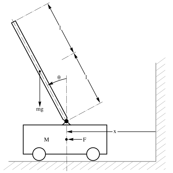
pendssm = StateSpaceModel[{{{0, 1, 0, 0}, {(g*(m + M))/
     (l*M), 0, 0, 0}, {0, 0, 0, 1},
   {(-g)*(m/M), 0, 0, 0}},
  {{0}, {-l^(-1)/M}, {0}, {M^(-1)}},
{{1, 0, 0, 0}, {0, 0, 1, 0}}, {{0}, {0}}}, SamplingPeriod -> None, SystemsModelLabels -> None] /. {M -> 5.6, m -> 0.53, l -> 0.85, g -> 9.8};{q, r} = {(| | | | |
| -- | - | -- | - |
| 10 | 0 | 0 | 0 |
| 0 | 1 | 0 | 0 |
| 0 | 0 | 10 | 0 |
| 0 | 0 | 0 | 1 |), (1000)};Subscript[s, init] = (| |
| --- |
| 0 |
| 0 |
| 0.1 |
| 0 |);x = RiccatiSolve[Normal[pendssm][[1 ;; 2]], {q, r}];Subscript[J, opt] = (Transpose[Subscript[s, init]].x.Subscript[s, init])[[1, 1]]Obtain the cost by numerical integration:
k = LQRegulatorGains[pendssm, {q, r}];Subscript[ss, CL] = SystemsModelStateFeedbackConnect[pendssm, k];Subscript[x, t] = StateResponse[{Subscript[ss, CL], Flatten[Subscript[s, init]]}, {0}, {t, 10^5}];Subscript[J, opt] = NIntegrate[Subscript[x, t].(q + Transpose[k].r.k).Subscript[x, t], {t, 0, 10^5}]Track the "cost to go" at each instant along the optimal trajectory:
Plot[Evaluate[Subscript[x, t].x.Subscript[x, t]], {t, 0, 50}, PlotRange -> All]Compute an optimal state-feedback gain that places all closed-loop poles to the left of ![]() :
:
{a, b, q, r} = {(| | | | | |
| ---- | ---- | ----- | ----- | --- |
| -0.2 | 0.5 | 0 | 0 | 0 |
| 0 | -0.5 | 1.6 | 0 | 0 |
| 0 | 0 | -14.3 | 85.8 | 0 |
| 0 | 0 | 0 | -33.3 | 100 |
| 0 | 0 | 0 | 0 | -10 |), (| |
| -- |
| 0 |
| 0 |
| 0 |
| 0 |
| 30 |), (| | | | | |
| -- | -- | - | - | - |
| 10 | 0 | 0 | 0 | 0 |
| 0 | 20 | 0 | 0 | 0 |
| 0 | 0 | 6 | 0 | 0 |
| 0 | 0 | 0 | 2 | 0 |
| 0 | 0 | 0 | 0 | 5 |), (1)};Subscript[a, 1] = a + α IdentityMatrix[Length[a]] /. α -> 2;k = Inverse[r].Transpose[b].RiccatiSolve[{Subscript[a, 1], b}, {q, r}];Eigenvalues[a - b.k]The closed-loop poles without any prescribed degree of stability:
Eigenvalues[a - b.(Inverse[r].Transpose[b].RiccatiSolve[{a, b}, {q, r}])]Compute the minimum error covariance for a Kalman estimator:
{a, b, c, w, v} = {(| | | |
| ---- | ---- | --- |
| -1.7 | 50 | 260 |
| 0.22 | -1.4 | -32 |
| 0 | 0 | -12 |), (| | | |
| ---- | ------- | ----- |
| -272 | 0.02 | 0.1 |
| 0 | -0.0035 | 0.004 |
| 14 | 0 | 0 |), (| | | |
| - | - | - |
| 1 | 0 | 0 |
| 0 | 1 | 0 |), (| | |
| -- | -- |
| 10 | 0 |
| 0 | 10 |), (| | |
| - | - |
| 1 | 0 |
| 0 | 1 |)};g = b[[All, {2, 3}]];q = g.v.Transpose[g];Tr[RiccatiSolve[{Transpose[a], Transpose[c]}, {q, v}]]Properties & Relations (8)
Find the optimal gains with cross-coupling matrix p:
{a, b} = {(| | |
| ------------------ | ------------------ |
| 2.5731 + 0.3269 I | 0.725 - 0.3024 I |
| -0.9543 - 2.7184 I | -2.5731 - 0.3268 I |), (| | |
| ----------------- | ----------------- |
| -0.1076 - 0.2184I | -0.835 - 0.0684 I |
| -0.6379 + 1.198I | 0.08 + 0.6334I |)};{q, r, p} = {(| | |
| - | - |
| 2 | 0 |
| 0 | 4 |), (| | |
| ----- | ----- |
| 1 | 1 - I |
| 1 + I | 1 |), (| | |
| - | - |
| 4 | 1 |
| 3 | 2 |)};x = RiccatiSolve[{a, b}, {q, r, p}];An equivalent result can be found be incorporating p into the a and q matrices:
xp = RiccatiSolve[{a - b.Inverse[r].ConjugateTranspose[p], b}, {q - p.Inverse[r].ConjugateTranspose[p], r}];xp - x//ChopIf {a,b} is controllable and {a,g} is observable, and q=Transpose[g].g, then the solution to the Riccati equation is positive definite:
{a, b, g, r} = {(| | | | | |
| ---- | ----- | ------ | ------ | ----- |
| 0.98 | 0.048 | 0.0025 | 0.0046 | 0.008 |
| 0 | 0.95 | 0.08 | 0.2 | 0.533 |
| 0 | 0 | 0.23 | 1.26 | 6.52 |
| 0 | 0 | 0 | 0.082 | 1.428 |
| 0 | 0 | 0 | 0 | 0.367 |), (| |
| ------ |
| 0.0059 |
| 0.509 |
| 10.15 |
| 3.97 |
| 1.89 |), (1 0 0 0 0), (1)};{ControllableModelQ[StateSpaceModel[{a, b}]], ControllableModelQ[StateSpaceModel[{Transpose[a], Transpose[g]}]]}PositiveDefiniteMatrixQ[RiccatiSolve[{a, b}, {Transpose[g].g, r}]]The eigenvalues of the Hamiltonian matrix ![]() are pairs of the form {λ,-λ}:
are pairs of the form {λ,-λ}:
With[{a = (| | |
| -------------------- | ------------------- |
| -16.826 - 18.09129 I | 6.1228 - 28.4026 I |
| 19.2776 - 1.14335 I | 13.826 + 18.0913 I |), b = (| |
| ------------------ |
| -0.8019 - 0.0491 I |
| 0.4257 - 0.4331 I |), q = (| | |
| -- | - |
| 10 | 0 |
| 0 | 1 |), r = (1)}, H = ArrayFlatten[(| | |
| -- | ----------------------------------- |
| a | -b.Inverse[r].ConjugateTranspose[b] |
| -q | -ConjugateTranspose[a] |)]];ListPlot[Eigenvalues[H] /. Complex[x_, y_] :> {x, y}, PlotStyle -> PointSize[Medium]]Complement[Eigenvalues[H], Eigenvalues[-H], SameTest -> (Chop[#1 - #2] == 0&)]The ability to obtain a stabilizing solution depends on the Hamiltonian matrix:
{a, b, q, r} = {(| | |
| - | - |
| 3 | 0 |
| 0 | 3 |), (| | |
| - | - |
| 1 | 0 |
| 0 | 1 |), (| | |
| - | - |
| 1 | 0 |
| 0 | 1 |), (| | |
| - | - |
| 1 | 0 |
| 0 | 1 |)};{vals, vecs} = Eigensystem[ArrayFlatten[(| | |
| -- | -------------------------- |
| a | -b.Inverse[r].Transpose[b] |
| -q | -Transpose[a] |)]]The Hamiltonian matrix must satisfy the stability property:
Cases[vals, Complex[0, _]]As well as the complementarity property:
stableBasis = Extract[vecs, Position[vals, _ ? (# < 0&), {1}]];{{Subscript[x, 1], Subscript[x, 2]}} = Partition[stableBasis, {2, 2}]MatrixRank[Subscript[x, 1]] == 2Subscript[x, 2].Inverse[Subscript[x, 1]]//SimplifyRiccatiSolve[{a, b}, {q, r}] == %Find the eigenvalues of the feedback system with ![]() :
:
{a, b, q, r} = {(| | |
| -- | -- |
| 7 | 10 |
| -5 | -8 |), (| |
| ------ |
| (5/3) |
| -(4/3) |), (| | |
| --- | --- |
| 0.3 | 0 |
| 0 | 0.9 |), (0.5)};Eigenvalues[a - b.Inverse[r].Transpose[b].RiccatiSolve[{a, b}, {q, r}]]These are also the stable eigenvalues of the Hamiltonian matrix:
λ = Eigenvalues[ArrayFlatten[(|    |                            |
| -- | -------------------------- |
| a  | -b.Inverse[r].Transpose[b] |
| -q | -Transpose[a] |)]];Select[λ, # < 0&]Compute optimal state feedback gains using RiccatiSolve:
{a, b, q, r} = {(| | |
| - | - |
| 0 | 1 |
| 0 | 0 |), (| |
| - |
| 0 |
| 1 |), (| | |
| - | - |
| 1 | 0 |
| 0 | 1 |), (1)};Inverse[r].Transpose[b].RiccatiSolve[{a, b}, {q, r}]//N//ChopUse LQRegulatorGains to compute the same result directly:
LQRegulatorGains[StateSpaceModel[{a, b}], {q, r}]//N//ChopCompute optimal output feedback gains using RiccatiSolve:
{a, b, c, q, r} = {(| | | |
| -- | -- | -- |
| -2 | 0 | 1 |
| 0 | -1 | 0 |
| -3 | -4 | -2 |), (| | |
| - | - |
| 0 | 1 |
| 0 | 0 |
| 1 | 0 |), (| | | |
| - | - | - |
| 1 | 0 | 0 |
| 0 | 1 | 0 |), (| | |
| --- | --- |
| 100 | 0 |
| 0 | 0.1 |), (| | |
| - | - |
| 1 | 0 |
| 0 | 1 |)};Inverse[r].Transpose[b].RiccatiSolve[{a, b}, {Transpose[c].q.c, r}]//MatrixFormLQOutputRegulatorGains gives the same result:
LQOutputRegulatorGains[StateSpaceModel[{a, b, c}], {q, r}]//MatrixFormCompute optimal estimator gains using RiccatiSolve:
{a, b, c} = {(|       |       |      |     |
| ----- | ----- | ---- | --- |
| -0.02 | 0.005 | 2.4  | -32 |
| -0.14 | 0.44  | -1.3 | 30  |
| 0     | 0.018 | -1.6 | 1.2 |
| 0     | 0     | 1    | 0   |), (|      |       |
| ---- | ----- |
| 0.14 | -0.12 |
| 0.36 | -0.86 |
| 0.35 | 0.009 |
| 0 | 0 |), (0 1 0 0)};w = 10^-2(| | |
| - | - |
| 1 | 0 |
| 0 | 1 |);v = ((1/10000));RiccatiSolve[{Transpose[a], Transpose[c]}, {b.w.Transpose[b], v}].Transpose[c].Inverse[v]Use LQEstimatorGains to compute this result directly:
LQEstimatorGains[StateSpaceModel[{a, b, c}], {w, v}]Possible Issues (1)
If ![]() is not stabilizable or
is not stabilizable or ![]() is not detectable, then the Riccati equation with
is not detectable, then the Riccati equation with ![]() has no stabilizing solution:
has no stabilizing solution:
{a, b, g, r} = {(| | | |
| - | -- | - |
| 1 | 0 | 0 |
| 1 | -1 | 1 |
| 0 | 0 | 2 |), (| |
| - |
| 1 |
| 1 |
| 0 |), (1 0 0), (1)};{ControllableModelQ[StateSpaceModel[{a, b}]], ControllableModelQ[StateSpaceModel[{Transpose[a], Transpose[g]}]]}RiccatiSolve[{a, b}, {Transpose[g].g, r}]Text
Wolfram Research (2010), RiccatiSolve, Wolfram Language function, https://reference.wolfram.com/language/ref/RiccatiSolve.html (updated 2014).
CMS
Wolfram Language. 2010. "RiccatiSolve." Wolfram Language & System Documentation Center. Wolfram Research. Last Modified 2014. https://reference.wolfram.com/language/ref/RiccatiSolve.html.
APA
Wolfram Language. (2010). RiccatiSolve. Wolfram Language & System Documentation Center. Retrieved from https://reference.wolfram.com/language/ref/RiccatiSolve.html