

MagneticSymmetryValue
MagneticSymmetryValue[pred,vars,pars]
represents a magnetic symmetry boundary condition for PDEs with predicate pred indicating where it applies, with model variables vars and global parameters pars.
MagneticSymmetryValue[pred,vars,pars,lkey]
represents a magnetic symmetry boundary condition with local parameters specified in pars[lkey].
Details
- MagneticSymmetryValue specifies a symmetry boundary condition for MagnetostaticPDEComponent.
- MagneticSymmetryValue specifies a boundary condition for MagnetostaticPDEComponent and is used as part of the modeling equation:
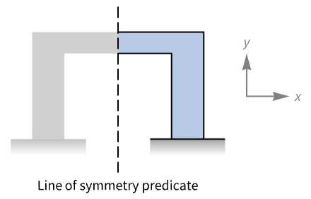
- MagneticSymmetryValue is typically used to model a boundary with mirror symmetry along an axis.
- MagneticSymmetryValue models a boundary with mirror symmetry with dependent variable
 and independent variables
  .
. - Stationary variables vars are vars={Vm[x1,…,xn],{x1,…,xn}}.
- The linear form of MagnetostaticPDEComponent with vacuum permeability
 in units of [
![TemplateBox[{InterpretationBox[, 1], {"H", , "/", , "m"}, henries per meter, {{(, "Henries", )}, /, {(, "Meters", )}}}, QuantityTF]](Files/MagneticSymmetryValue.en/6.png "TemplateBox[{InterpretationBox[, 1], {\"H\", , \"/\", , \"m\"}, henries per meter, {{(, \"Henries\", )}, /, {(, \"Meters\", )}}}, QuantityTF]") ] and relative permeability
] and relative permeability  is given by:
 - MagneticSymmetryValue with boundary unit normal
 and
and  a magnetic flux density vector models:
 - Model parameters pars as specified as for MagnetostaticPDEComponent.
- MagneticSymmetryValue is effectively the same as MagneticFluxDensityValue with a magnetic flux of 0.
- The boundary predicate pred can be specified as in NeumannValue.
- If the MagneticSymmetryValue depends on parameters
 that are specified in the association pars as …,keypi…,pivi,…, the parameters
  are replaced with
  .
.
Examples
open all close allBasic Examples (1)
Scope (2)
Set up a magnetic symmetry boundary condition in 3D:
MagneticSymmetryValue[x ≥ 0, {Subscript[V, m][x, y, z], {x, y, z}}, <||>]Define model variables vars for a magnetic field with model parameters pars and a specific parameter boundary condition:
vars = {Subscript[V, m][x, y], {x, y}};
pars = <|"BoundaryCondition1" -> <||>|>;
Evaluate the boundary condition:
MagneticSymmetryValue[x == 1 / 5, vars, pars, "BoundaryCondition1"]Applications (1)
Model an iron cube embedded in air and emerged in a homogeneous magnetic field of ![]() [
[![]() ] directed along the
] directed along the ![]() axis. The domain is composed of an iron cube of length
axis. The domain is composed of an iron cube of length ![]() [
[![]() ]. Due to symmetry, only 1/8 of the whole domain is simulated. The air boundary surrounding the iron cube is modeled as a second cube of length
]. Due to symmetry, only 1/8 of the whole domain is simulated. The air boundary surrounding the iron cube is modeled as a second cube of length ![]() [
[![]() ].
].
In the reduced geometry, at the surfaces parallel to the planes ![]() -
-![]() and
and ![]() -
-![]() a symmetry boundary condition needs to be applied.
a symmetry boundary condition needs to be applied.
mesh = \!\(\*Graphics3DBox[«6»]\);The mesh has internal boundaries that represent the inner iron cube. Define the iron cube:
ironCube = Cuboid[{0, 0, 0}, {0.02, 0.02, 0.02}];Visualize a wireframe of the mesh:
Show[HighlightMesh[RegionBoundary[mesh], {}, PlotTheme -> "Lines"], Graphics3D[{Gray, ironCube}]]vars = {Vm[x, y, z], {x, y, z}};Define parameters the permeability of vacuum ![]() and iron
and iron ![]() :
:
pars = <|"RelativePermeability" -> Piecewise[{{1000.0, RegionMember[ironCube][{x, y, z}]}}, 1] * IdentityMatrix[3]|>;To specify the homogeneous magnetic field across the domain, an outward magnetic flux density ![]() normal to the boundary at
normal to the boundary at ![]() is specified.
is specified.
Set up the magnetic flux density condition:
Subscript[Γ, n] = MagneticFluxDensityValue[z == 0.1, vars, pars, <|"NormalMagneticFluxDensity" -> -1|>]Set up the magnetic symmetry condition:
Subscript[Γ, s] = MagneticSymmetryValue[x == 0 || y == 0, vars, pars]Since the magnetic symmetry condition is a Neumann zero boundary condition, which is the default boundary condition if nothing is specified on a boundary, it could also be omitted.
Solve the magnetostatic PDE model:
VmFun = NDSolveValue[{MagnetostaticPDEComponent[vars, pars] == Subscript[Γ, n] + Subscript[Γ, s], MagneticPotentialCondition[z == 0, vars, pars, <||>]}, Vm, {x, y, z}∈mesh]Compute the magnetic field intensity:
HField = -Grad[VmFun[x, y, z], {x, y, z}];To visualize another 1/8 of the field, at ![]() , the symmetric behavior of the field must be considered. At positive
, the symmetric behavior of the field must be considered. At positive ![]() values, the field is
values, the field is ![]() and at negative
and at negative ![]() values, the field is
values, the field is ![]() .
.
Visualize the symmetric vector field at ![]() of the complete geometry:
of the complete geometry:
Show[Graphics3D[...], HighlightMesh[...], VectorPlot3D[Evaluate[Piecewise[{{{-1, 1, 1} * HField /. x -> Abs@x, x < 0}}, HField /. x -> Abs@x]], {x, -0.1, 0.1}, {y, 0, 0.1}, {z, 0, 0.1}, VectorPoints -> 8]]Text
Wolfram Research (2025), MagneticSymmetryValue, Wolfram Language function, https://reference.wolfram.com/language/ref/MagneticSymmetryValue.html.
CMS
Wolfram Language. 2025. "MagneticSymmetryValue." Wolfram Language & System Documentation Center. Wolfram Research. https://reference.wolfram.com/language/ref/MagneticSymmetryValue.html.
APA
Wolfram Language. (2025). MagneticSymmetryValue. Wolfram Language & System Documentation Center. Retrieved from https://reference.wolfram.com/language/ref/MagneticSymmetryValue.html