Wolfram Language & System Documentation Center

MassConcentrationCondition

MassConcentrationCondition[pred,vars,pars]

represents a mass concentration boundary condition for PDEs with predicate pred indicating where it applies, with model variables vars and global parameters pars.

MassConcentrationCondition[pred,vars,pars,lkey]

represents a thermal surface boundary condition with local parameters specified in pars[lkey].

Details

MassConcentrationCondition specifies a boundary condition for MassTransportPDEComponent.
MassConcentrationCondition is typically used to set a mass species concentration on the boundary. Common examples include a mass species inflow condition.

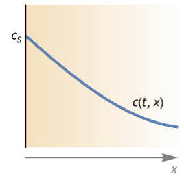
MassConcentrationCondition sets a specific mass species concentration on the boundary with dependent variable in [ $TemplateBox[{InterpretationBox[, 1], {"mol", , "/", , {"m", ^, 3}}, moles per meter cubed, {{(, "Moles", )}, /, {(, {"Meters", ^, 3}, )}}}, QuantityTF]$ ], independent variables in [] and time variable in [].
Stationary variables vars are vars={c[x₁,…,x_n],{x₁,…,x_n}}.
Time-dependent variables vars are vars={c[t,x₁,…,x_n],t,{x₁,…,x_n}}.
The mass concentration condition MassConcentrationCondition models .

Model parameters pars as specified for MassTransportPDEComponent.
The following additional model parameters pars can be given:
parameter default symbol

"MassConcentration" 0 , mass concentration [ $TemplateBox[{InterpretationBox[, 1], {"mol", , "/", , {"m", ^, 3}}, moles per meter cubed, {{(, "Moles", )}, /, {(, {"Meters", ^, 3}, )}}}, QuantityTF]$ ]
MassConcentrationCondition evaluates to a DirichletCondition.
The boundary predicate pred can be specified as in DirichletCondition.
If the MassConcentrationCondition depends on parameters that are specified in the association pars as …,keyp_i…,p_iv_i,…, the parameters are replaced with .

Examples

open all close all

Basic Examples (2)

Set up a mass concentration boundary condition:

Wolfram Language code: MassConcentrationCondition[x ≥ 0, {c[t, x, y], t, {x, y}}, <|"MassConcentration" -> Subscript[c, s][t, x, y]|>]

Set up a system of mass concentration boundary conditions:

Wolfram Language code:

MassConcentrationCondition[x ≥ 0, {{Subscript[c, 1][x], Subscript[c, 2][x]}, {x}}, <|"MassConcentration" -> {Subscript[c, s1][x], Subscript[c, s2][x]}|>]

Scope (7)

Basic Uses (2)

Define model variables vars for a transient species field with model parameters pars and a specific boundary condition parameter:

Wolfram Language code:

vars = {c[t, x, y], t, {x, y}};
pars = <|"DiffusionCoefficient" -> 0.026, "MassConvectionVelocity" -> {0.1}, "BoundaryCondition1" -> <|"MassConcentration" -> c1|>|>;
MassConcentrationCondition[x == 1, vars, pars, "BoundaryCondition1"]

Define model variables vars for a transient species field with model parameters pars and multiple specific parameter boundary conditions:

Wolfram Language code:

vars = {c[t, x, y], t, {x, y}};
	
pars = <|"DiffusionCoefficient" -> 0.026, "MassConvectionVelocity" -> {0.1}, "BoundaryCondition1" -> <|"MassConcentration" -> c1|>, "BoundaryCondition2" -> <|"MassConcentration" -> c2|>|>;

Wolfram Language code: MassConcentrationCondition[x == 0, vars, pars, "BoundaryCondition1"]

Wolfram Language code: MassConcentrationCondition[x == 1, vars, pars, "BoundaryCondition2"]

1D (1)

Model a 1D chemical species field in an incompressible fluid whose right side and left side are subjected to a mass concentration and inflow condition, respectively:

Set up the stationary mass transport model variables :

Wolfram Language code: vars = {c[x], {x}};

Set up a region :

Wolfram Language code: Ω = Line[{{0}, {1}}];

Specify the mass transport model parameters species diffusivity and fluid flow velocity :

Wolfram Language code: pars = <|"DiffusionCoefficient" -> 0.026, "MassConvectionVelocity" -> {0.1}|>;

Specify a species flux boundary condition:

Wolfram Language code: Subscript[Γ, flux] = MassFluxValue[x == 0, vars, pars, <|"MassFlux" -> 1|>]

Specify a mass concentration boundary condition:

Wolfram Language code: Subscript[Γ, C] = MassConcentrationCondition[x == 1, vars, pars, <|"MassConcentration" -> 0|>]

Set up the equation:

Wolfram Language code: eqn = MassTransportPDEComponent[vars, pars] == Subscript[Γ, flux]

Solve the PDE:

Wolfram Language code: cfun = NDSolveValue[{eqn, Subscript[Γ, C]}, c, x∈Ω];

Visualize the solution:

Wolfram Language code: Plot[cfun[x], x∈Ω, Rule[...]]

2D (1)

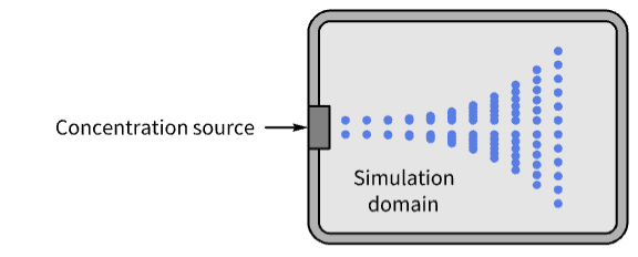
Model mass transport of a pollutant in a 2D rectangular region in an isotropic homogeneous medium. Initially, the pollutant concentration is zero throughout the region of interest. A concentration of 3000 is maintained at a strip with dimension 0.2 located at center of the left boundary, while the right boundary is subject to a parallel species flow with constant concentration of 1500 , allowing for mass transfer. A pollutant outflow of 100 is applied at both the top and bottom boundaries. A diffusion coefficient of 0.833 is distributed uniformly with a uniform horizontal velocity of 0.01 :

Set up the mass transport model variables :

Wolfram Language code: vars = {c[x, y], {x, y}};

Set up a rectangular domain with a width of and a height of :

Wolfram Language code: Ω = Rectangle[{0, 0}, {20, 10}];

Specify model parameters species diffusivity and fluid flow velocity :

Wolfram Language code: pars = <|"DiffusionCoefficient" -> 0.833, "MassConvectionVelocity" -> {0.01, 0}|>;

Set up a species concentration source of 0.2 in length at the center of the left surface:

Wolfram Language code:

Subscript[Γ, concentration] = MassConcentrationCondition[x == 0 && y ≤ 5.1 && y ≥ 4.9, vars, pars, <|"MassConcentration" -> 3000|>]

Set up a mass transfer boundary on the right surface:

Wolfram Language code:

Subscript[Γ, transfer] = MassTransferValue[x == 20, vars, pars, <|"AmbientConcentration" -> 1500, "MassTransferCoefficient" -> 5|>]

Set up an outflow flux q of on the top and bottom surfaces:

Wolfram Language code: Subscript[Γ, flux] = MassFluxValue[y == 0 || y == 10, vars, pars, <|"MassFlux" -> -100|>]

Set up the equation:

Wolfram Language code: eqn = MassTransportPDEComponent[vars, pars] == Subscript[Γ, transfer] + Subscript[Γ, flux]

Solve the PDE:

Wolfram Language code: cfun = NDSolveValue[{eqn, Subscript[Γ, concentration]}, c, {x, y}∈Ω];

Visualize the solution:

Wolfram Language code: ContourPlot[cfun[x, y], {x, y}∈Ω, ...]

3D (1)

Model a non-conservative chemical species field in a unit cubic domain, with two mass conditions at two lateral surfaces and a mass inflow through a circle with radius 0.2 at the center of the top surface, as well as an orthotropic mass diffusivity :

del .(-d del c(x,y,z))+v^->.del c(x,y,z)^(︷^( mass transport model )) =|_(Gamma_(z=1& (x-0.5)^2+(y-0.5)^2<=0.04))q(x,y,z)^(︷^( mass flux value ))

Set up the mass transport model variables :

Wolfram Language code: vars = {c[x, y, z], {x, y, z}};

Set up a region :

Wolfram Language code: Ω = Cuboid[{0, 0, 0}, {1, 1, 1}];

Specify a diffusivity and a flow velocity field :

Wolfram Language code: pars = <|"DiffusionCoefficient" -> {{1, 0, 0}, {0, 5, 0}, {0, 0, 10}}, "MassConvectionVelocity" -> {0, 10, 0}|>;

Specify mass concentrations:

Wolfram Language code:

Subscript[Γ, CC] = {MassConcentrationCondition[x == 0, vars, <|"MassConcentration" -> 0|>], MassConcentrationCondition[x == 1, vars, <|"MassConcentration" -> 1|>]}

Specify a flux condition of through a regional circle on the top surface:

Wolfram Language code: Subscript[Γ, flux] = MassFluxValue[z == 1 && (x - 0.5) ^ 2 + (y - 0.5) ^ 2 ≤ 0.04, vars, pars, <|"MassFlux" -> 100|>]

Set up the equation:

Wolfram Language code: eqn = MassTransportPDEComponent[vars, pars] == Subscript[Γ, flux]

Solve the PDE:

Wolfram Language code: cfun = NDSolveValue[{eqn, Subscript[Γ, CC]}, c, {x, y, z}∈Ω];

Visualize the solution:

Wolfram Language code: GraphicsRow[Table[SliceContourPlot3D[cfun[x, y, z], sl, {x, y, z}∈Ω, ...], {...}]]

Material Regions (1)

Model a 1D chemical species transport through different material with a reaction rate in one. The right side and left side are subjected to a mass concentration and inflow condition, respectively:

Set up the stationary mass transport model variables :

Wolfram Language code: vars = {c[x], {x}};

Set up a region :

Wolfram Language code: Ω = Line[{{0}, {1}}];

Specify the mass transport model parameters species diffusivity and a reaction rate active in the region :

Wolfram Language code: pars = <|"DiffusionCoefficient" -> 0.01, "MassReactionRate" -> If[x > 1 / 2, 1, 0]|>;

Specify a species flux boundary condition:

Wolfram Language code: Subscript[Γ, flux] = MassFluxValue[x == 0, vars, pars, <|"MassFlux" -> 1|>]

Specify a mass concentration boundary condition:

Wolfram Language code: Subscript[Γ, C] = MassConcentrationCondition[x == 1, vars, pars, <|"MassConcentration" -> 0|>]

Set up the equation:

Wolfram Language code: eqn = MassTransportPDEComponent[vars, pars] == Subscript[Γ, flux]

Solve the PDE:

Wolfram Language code: cfun = NDSolveValue[{eqn, Subscript[Γ, C]}, c, x∈Ω];

Visualize the solution:

Wolfram Language code: Show[Plot[cfun[x], x∈Ω, Rule[...]], Graphics[...]]

Nonlinear Time Dependent (1)

Model a 1D non-conservative chemical species field with a nonlinear diffusivity coefficient and an outflow condition through part of the boundary, which is expressed as follows:

Set up the mass transport model variables :

Wolfram Language code: vars = {c[t, x], t, {x}};

Set up a region :

Wolfram Language code: Ω = Line[{{0}, {1}}];

Specify a nonlinear species diffusivity and fluid flow velocity :

Wolfram Language code: pars = <|"DiffusionCoefficient" -> {{0.001 * Log[c[t, x] ^ 2 + 1]}}, "MassConvectionVelocity" -> {0.02}|>;

Specify an outflow flux of applied at the right end:

Wolfram Language code: Subscript[Γ, flux] = MassFluxValue[x == 1, vars, pars, <|"MassFlux" -> -1|>]

Specify a time-dependent mass concentration surface condition:

Wolfram Language code: Subscript[Γ, C] = MassConcentrationCondition[x == 0, vars, pars, <|"MassConcentration" -> 100 + 0.1 * t|>]

Set up an initial condition:

Wolfram Language code: ics = c[0, x] == 100;

Set up the equation:

Wolfram Language code: eqn = MassTransportPDEComponent[vars, pars] == Subscript[Γ, flux]

Solve the PDE:

Wolfram Language code: cfun = NDSolveValue[{eqn, ics, Subscript[Γ, C]}, c, {t, 0, 500}, x∈Ω];

Visualize the solution:

Wolfram Language code: Manipulate[Show[Plot[cfun[t, x], ...], Graphics[...]], {{t, 30}, 0, 500, 1}, Rule[...]]

Applications (2)

Compute the mass concentration with model variables and parameters with a mass concentration of at the left boundary:

Wolfram Language code:

vars = {c[t, x], t, {x}};
pars = <|"MassDiffsivity" -> 0.026, "MassConcentration" -> Sin[π t / 300]|>;

Set up the equation:

Wolfram Language code: eqn = {MassTransportPDEComponent[vars, pars] == 0, MassConcentrationCondition[x == 0, vars, pars]}

Solve the PDE:

Wolfram Language code: cfun = NDSolveValue[{eqn, c[0, x] == 0}, c, {t, 0, 600}, x∈Line[{{0}, {1 / 5}}]];

Visualize the solution and note the sinusoidal mass change on the left:

Wolfram Language code: Manipulate[Plot[Tfun[t, x], {x, 0, 1 / 5}, ...], {{t, 360}, 0, 600, 20}, Rule[...]]

Model mass transport of a pollutant in a 2D rectangular region in an isotropic homogeneous medium. Initially, the pollutant concentration is zero throughout the region of interest. A concentration of 3000 is maintained at a strip with dimension 0.2 located at center of left boundary, while a pollutant outflow of 100 is applied at both the top and bottom boundaries. A diffusion coefficient of 0.833 is distributed uniformly, but both horizontal and vertical velocity are spatial dependent:

Set up the mass transport model variables :

Wolfram Language code: vars = {c[x, y], {x, y}};

Set up a rectangular domain with a width of and a height of :

Wolfram Language code: Ω = Rectangle[{0, 0}, {20, 10}];

Specify model parameters species diffusivity and fluid flow velocity :

Wolfram Language code: pars = <|"DiffusionCoefficient" -> 0.833, "MassConvectionVelocity" -> {0.01x ^ 2, -0.02y}|>;

Set up a species concentration source of 0.2 in length at the center of the left surface:

Wolfram Language code: Subscript[Γ, C] = MassConcentrationCondition[x == 0 && 4.9 ≤ y ≤ 5.1, vars, pars, <|"MassConcentration" -> 3000|>]

Set up an outflow flux of on the top and bottom surfaces:

Wolfram Language code: Subscript[Γ, flux] = MassFluxValue[y == 0 || y == 10, vars, pars, <|"MassFlux" -> -10|>]

Set up the equation:

Wolfram Language code: eqn = {MassTransportPDEComponent[vars, pars] == Subscript[Γ, flux], Subscript[Γ, C]}

Solve the PDE:

Wolfram Language code: cfun = NDSolveValue[eqn, c, {x, y}∈Ω];

Visualize the solution:

Wolfram Language code: ContourPlot[cfun[x, y], {x, y}∈Ω, Rule[...]]

Top

More Learning

Tech Support

Wolfram Solutions

Wolfram Solutions For Education

Get Started

Grow Your Skills

Work with Us

Educational Programs for Adults

Educational Programs for Youth

Read

MassConcentrationCondition

Details

Examples

Basic Examples (2)

Scope (7)

Basic Uses (2)

1D (1)

2D (1)

3D (1)

Material Regions (1)

Nonlinear Time Dependent (1)

Applications (2)

Text

CMS

APA

BibTeX

BibLaTeX

	parameter	default	symbol
	"MassConcentration"	0	, mass concentration [ $TemplateBox[{InterpretationBox[, 1], {"mol", , "/", , {"m", ^, 3}}, moles per meter cubed, {{(, "Moles", )}, /, {(, {"Meters", ^, 3}, )}}}, QuantityTF]$ ]

MassConcentrationCondition

Details

Examples

Basic Examples (2)

Scope (7)

Basic Uses (2)

1D (1)

2D (1)

3D (1)

Material Regions (1)

Nonlinear Time Dependent (1)

Applications (2)

See Also

Tech Notes

Related Guides

History

Text

CMS

APA

BibTeX

BibLaTeX