

NuttallWindow
represents a Nuttall window function of x.
Details
- NuttallWindow is a window function typically used in signal processing applications where data needs to be processed in short segments.
- Window functions have a smoothing effect by gradually tapering data values to zero at the ends of each segment.
- NuttallWindow[x] is equal to
![ (121849 cos(2 pi x)+36058 cos(4 pi x)+3151 cos(6 pi x)+88942)/(250000) -1/2<=x<=1/2; 0 TemplateBox[{x}, Abs]>1/2;](Files/NuttallWindow.en/2.png " (121849 cos(2 pi x)+36058 cos(4 pi x)+3151 cos(6 pi x)+88942)/(250000) -1/2<=x<=1/2; 0 TemplateBox[{x}, Abs]>1/2;") .
. - NuttallWindow automatically threads over lists.
Examples
open all close allBasic Examples (3)
Plot[NuttallWindow[x], {x, -1, 1}]Plot3D[NuttallWindow[x]NuttallWindow[y], {x, -1, 1}, {y, -1, 1}, PlotRange -> All, Exclusions -> None]Extract the continuous function representing the Nuttall window:
FunctionExpand[NuttallWindow[x]]Scope (4)
NuttallWindow[0.1]Translated and dilated Nuttall window:
Plot[NuttallWindow[(x - 1) / 2], {x, -1, 3}]2D Nuttall window with a circular support:
Plot3D[NuttallWindow[Sqrt[x ^ 2 + y ^ 2]], {x, -1, 1}, {y, -1, 1}, PlotRange -> All, Exclusions -> None]Discrete Nuttall window of length 15:
ListPlot[Array[NuttallWindow, 15, {-1 / 2, 1 / 2}], Filling -> Axis]Discrete 15×10 2D Nuttall window:
ListPointPlot3D[Array[NuttallWindow[#1] NuttallWindow[#2]&, {15, 10}, {{-1 / 2, 1 / 2}}], Filling -> Axis, PlotRange -> All]Applications (3)
Create a moving-average filter of length 11:
h = ConstantArray[1 / 11., 11]Taper the filter using a Nuttall window:
w = Array[NuttallWindow, Length[h], {-1 / 2, 1 / 2}];
fir = w h / Total[w h];
Log-magnitude plot of the power spectra of the filters:
Plot[Evaluate[20Log10[Abs@ListFourierSequenceTransform[#, ω]]& /@ {h, fir}], {ω, 0.1, Pi}, PlotRange -> {5, -120}, GridLines -> Automatic]Use a window specification to calculate sample PowerSpectralDensity:
proc = ARMAProcess[1, {.5}, {.3}, 1];
data = RandomFunction[proc, {50}];spec = PowerSpectralDensity[data, w, NuttallWindow];Compare to spectral density calculated without a windowing function:
sd = PowerSpectralDensity[data, w];sd === specThe plot shows that window smooths the spectral density:
Plot[{sd, spec}, {w, -π, π}, PlotRange -> All, PlotLegends -> {"no window", "with window"}]Compare to the theoretical spectral density of the process:
Plot[{spec, Evaluate@PowerSpectralDensity[proc, w]}, {w, -π, π}, PlotLegends -> {"data", "process"}]Use a window specification for time series estimation:
data = RandomFunction[ARMAProcess[1, {.3}, {.4}, 1], {300}];Specify window for spectral estimator:
EstimatedProcess[data, ARMAProcess[1, 1], ProcessEstimator -> {"SpectralEstimator", "Window" -> NuttallWindow}]Properties & Relations (3)
The area under the Nuttall window:
area = Integrate[NuttallWindow[x], {x, -∞, ∞}]Normalize to create a window with unit area:
Plot[{NuttallWindow[x], NuttallWindow[x] / area}, {x, -1, 1}, PlotRange -> All]Fourier transform of the Nuttall window:
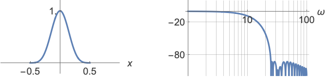
f = FourierTransform[NuttallWindow[x], x, w]Power spectrum of the Nuttall window:
LogLinearPlot[20 Log[10, Abs[f]], {w, .1, 100}]The Nuttall window has a continuous derivative:
der = D[NuttallWindow[x], x]Plot[der, {x, -1, 1}]Text
Wolfram Research (2012), NuttallWindow, Wolfram Language function, https://reference.wolfram.com/language/ref/NuttallWindow.html.
CMS
Wolfram Language. 2012. "NuttallWindow." Wolfram Language & System Documentation Center. Wolfram Research. https://reference.wolfram.com/language/ref/NuttallWindow.html.
APA
Wolfram Language. (2012). NuttallWindow. Wolfram Language & System Documentation Center. Retrieved from https://reference.wolfram.com/language/ref/NuttallWindow.html