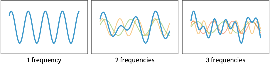
PeriodicModel represents a sinusoidal function in the given variable in a format suitable for symbolic or numerical evaluation and fitting.
Periodic models describe repeating phenomena such as oscillations, wave motion, alternating currents and seasonal or cyclic variations.

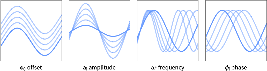
PeriodicModel[n] is parametrized as $sum_(i=1)^nTemplateBox[{i}, CTraditional] sin(x TemplateBox[{{i, +, 1}}, CTraditional]+TemplateBox[{{i, +, 2}}, CTraditional])+TemplateBox[{0}, CTraditional]$ . The number of parameters is therefore equal to .
When used in ModelFit, the coefficients of the n periodic functions are first estimated individually to obtain starting values for FindFit.

Hyperparameters

The following hyperparameters may be specified to control the fit:
"FrequencyCount" 1 number of frequencies n

"SamplePoints" 10 initial number of search points for each frequency
Possible settings for the number of frequencies include:

	i	number of frequencies to fit
	UpTo[n]	all i up to and including n
	n;;m	all i between n and m inclusive
	n;;m;;s	all i between n and m in steps of s

Variables

When not specified, variables will automatically be enumerated using x[i].
Valid variable specifications vars include:
n the number of variables

symb a symbolic representation of a single variable

Parameters

When not specified, parameters will automatically be enumerated using C[0] for the constant offset, a[i] for the amplitudes, k[i] for the frequencies and ϕ[i] for the phase offsets.
Valid parameter pars specifications in the form {par₁,…} include:

	val	a fixed parameter value val
	par	a symbolic parameter name par
	parval	a symbolic name par set to a fixed value val
	{par,val₀}	a symbolic parameter named par with the initial value val₀

Properties

Model properties can be extracted using Information[PowerModel[…],prop].
Valid basic properties include:

	"BaseType"	model base type
	"Name"	model name
	"ShortName"	short identifier to use as label
	"InputType"	supported input types
	"OutputType"	supported output types

Valid data-related properties include:

	"ColumnNames"	names of the input features
	"ColumnVariableMap"	map between column names and model variables
	"InputSize"	dimensionality of the input
	"OutputSize"	dimensionality of the output
	"Trainable"	whether the model is fully specified and can be trained
	"Trained"	whether the model can be evaluated numerically
	"VariableColumnMap"	map between model variables and column names
	"Variables"	name of the model variables

Best model-related properties include:

	"Expression"	model expression
	"Function"	model as a pure function
	"SymbolicExpression"	model expression with symbolic parameters
	"TabularFunction"	pure function suitable to work on a tabular row

Parameter-related properties include:

	"Constraints"	parameter constraints
	"ParameterAssociation"	association of parameter names and values
	"ParameterCount"	the number of parameters
	"ParameterInitialValues"	initial values for the fit
	"ParameterNames"	parameter names
	"ParameterRules"	list of rules with parameter names and values
	"Parameters"	parameter values if present; names otherwise
	"ParameterValues"	parameter values

Hyperparameter-related properties include:

	"HyperparameterDefaultDomain"	default hyperparameter search domain
	"HyperparameterDomain"	specified hyperparameter search domain
	"Hyperparameters"	hyperparameter values

Examples

open all close all

Basic Examples (3)

Specify a generic periodic model:

Wolfram Language code: PeriodicModel[]

Specify the number of frequencies:

Wolfram Language code: PeriodicModel[2]

A model with a single frequency and t as the independent variable:

Wolfram Language code: PeriodicModel[1, t]

Use custom names for the symbolic parameters:

Wolfram Language code: PeriodicModel[1, {c, a, ω, ϕ}, t]

Plot over a variety of frequencies using constant parameters:

Wolfram Language code:

Plot[Evaluate@{PeriodicModel[1, {c -> 0, a -> 1, ω -> 1, ϕ -> 0}, 1][x], PeriodicModel[1, {c -> 1, a -> 1, ω -> 1.5, ϕ -> -1}, 1][x], PeriodicModel[1, {c -> 2, a -> 1, ω -> 2, ϕ -> -2}, 1][x]}, 
	{x, -2Pi, 2Pi}]

Scope (19)

Hyperparameters (4)

FrequencyCount (3)

Specify the number of frequencies of the model:

Wolfram Language code: PeriodicModel[2][x]

Use the name of the hyperparameter explicitly:

Wolfram Language code: PeriodicModel[<|"FrequencyCount" -> 2|>][x]

Specify a family of models with the maximum given number of frequencies:

Wolfram Language code: model = PeriodicModel[UpTo[2]]

Use ModelFit to find the best periodic model up to this maximum number of frequencies:

Wolfram Language code: ModelFit[1. + Sin[Range[10] + 0.1] + 0.5Cos[1.5 * Range[10]], model]

The number of frequencies is assumed to be one:

Wolfram Language code: ModelFit[1. + Sin[Range[10] + 0.1] + 0.5Cos[1.5 * Range[10]], PeriodicModel[]]

SamplePoints (1)

Specify the number of frequencies to search. Searching more frequencies improves the probability of finding the best one:

Wolfram Language code: ModelFit[{...}, PeriodicModel[<|"SamplePoints" -> 20, "FrequencyCount" -> 1|>]]

Variables (2)

Specify a PeriodicModel by degree alone:

Wolfram Language code: PeriodicModel[1]

Periodic models are always functions of a single variable:

Wolfram Language code: PeriodicModel[1][x]

Wolfram Language code: PeriodicModel[1][{x}]

Give the variable a custom symbolic representation:

Wolfram Language code: PeriodicModel[1, t]

Wolfram Language code: PeriodicModel[1, {t}]

These names are overwritten when the model is evaluated symbolically:

Wolfram Language code: PeriodicModel[1, t][a]

Wolfram Language code: PeriodicModel[1, {t}][{a}]

Parameters (3)

Parameter names are assigned automatically:

Wolfram Language code: PeriodicModel[3]

Specify custom parameter names:

Wolfram Language code: PeriodicModel[2, {c, a1, ω1, ϕ1, a2, ω2, ϕ2}, t]

The parameter list must have the correct length for the given number of frequencies:

Wolfram Language code: PeriodicModel[2, {c, a1, ω1, ϕ1, a2}, t]

Set a parameter to a specific value:

Wolfram Language code: PeriodicModel[1, {0, a, ω, ϕ}, t]

Specify a parameter name and set it to a constant value:

Wolfram Language code: PeriodicModel[1, {c -> 0, a, ω, ϕ}, t]

Wolfram Language code: Information[%, {"ParameterNames", "ParameterValues"}]

Evaluation (2)

Symbolically evaluate a single-variable model:

Wolfram Language code: PeriodicModel[1][x]

Wolfram Language code: PeriodicModel[1][{x}]

Evaluate a model on multiple different values:

Wolfram Language code: PeriodicModel[1][{Pi / 2, 2Pi}]

Wolfram Language code: PeriodicModel[1][{{x}, {y}}]

Information (4)

View general information about a model:

Wolfram Language code: Information[PeriodicModel[UpTo[2]]]

Some information is only available when variables or parameters are fully specified:

Wolfram Language code: Information[PeriodicModel[1, x]]

Extract a single property:

Wolfram Language code: Information[PeriodicModel[1, x], "Variables"]

View the available properties:

Wolfram Language code: Information[PeriodicModel[1, x], "Properties"]

Retrieve multiple properties:

Wolfram Language code: Information[PeriodicModel[2, x], {"Variables", "Parameters", "AngularFrequencies", "Frequencies", "PeriodLengths"}]

Fitting (4)

Fit a periodic model with a single Sin function:

Wolfram Language code: ModelFit[{...}, PeriodicModel[2]]

Attempt to fit up to three frequencies:

Wolfram Language code: ModelFit[{...}, PeriodicModel[UpTo[3]]]

View the report to compare the fits:

Wolfram Language code: ModelFit[{...}, PeriodicModel[UpTo[3]], "Report"]

Numerical parameter values are considered fixed during fitting:

Wolfram Language code: Information[ModelFit[{...}, PeriodicModel[1, {0, A, k, ϕ}, 1]], "ParameterValues"]

Fixing all the parameters will result in a model equivalent to the input:

Wolfram Language code: ModelFit[{...}, PeriodicModel[1, {0, 1, 2, 0}, 1], "ParameterValues"]

Compare the performance of a previously trained model with one trained on the actual data:

Wolfram Language code: report = ModelFit[{...}, {PeriodicModel[1, {0, 1, 2, 0}, 1], PeriodicModel[1]}, "Report"]

Compare the validation errors:

Wolfram Language code: report["ValidationLoss" -> All]

Extract the parameters for both models:

Wolfram Language code: report["ParameterValues" -> All]

Applications (2)

Monthly Temperature Variation (1)

Retrieve the daily temperature across five years:

Wolfram Language code: temperatures = WeatherData["KMDZ", "MeanTemperature", {{2015}, {2020}, "Day"}]

Fit a periodic model:

Wolfram Language code: model = ModelFit[temperatures, PeriodicModel[]]

Inspect the model fit:

Wolfram Language code: DateListPlot[{temperatures, AssociationMap[model[#]&, Normal@temperatures["Dates"]]}]

Sunspot Cycle (1)

To determine the cycle of the Wolf sunspot numbers, retrieve historical data:

Wolfram Language code: sunspotCount = ResourceData["Sample Data: Wolf Sunspot Numbers"]

Attempt a naive fit to the sunspot data:

Wolfram Language code: ModelFit[sunspotCount, PeriodicModel[]]

The fit fails because the frequencies present in the data are outside the normal search range. Increase the number of search points to search a wider range:

Wolfram Language code: defaultModel = ModelFit[sunspotCount, PeriodicModel[<|"SamplePoints" -> 20|>]]

Compare the plot to the data:

Wolfram Language code: DateListPlot[{sunspotCount, AssociationMap[defaultModel, sunspotCount["Dates"]]}, PlotRange -> All]

The default model has found the the single long period variation in the data, approximating the approximately 80-year Gleissberg cycle. Retrieve the frequency:

Wolfram Language code: frequency = Information[defaultModel, "Parameters"][[3]]

Fitting is performed on the renormalized dates; calculate the normalization factor:

Wolfram Language code: normalization = sunspotCount["LastDate"] - sunspotCount["FirstDate"]

And calculate the time period:

Wolfram Language code: timePeriod = UnitConvert[normalization * 2Pi / frequency, "Years"]

This is a little short for the Gleissberg cycle, potentially due to the short sampling period for such a low frequency, and any noise from the 11-year sunspot cycle. Fit additional sin waves to attempt to account for the shorter period:

Wolfram Language code: twoFrequencyModel = ModelFit[sunspotCount, PeriodicModel[2]]

Inspect the data:

Wolfram Language code:

DateListPlot[{sunspotCount, AssociationMap[defaultModel, sunspotCount["Dates"]], AssociationMap[twoFrequencyModel, sunspotCount["Dates"]]}, PlotRange -> All, PlotLegends -> {"Data", "Default", "2 frequency"}]

Calculate the frequencies of this plot:

Wolfram Language code: frequencies = Information[twoFrequencyModel, "Parameters"][[{3, 6}]]

You can see the 11-year sunspot cycle and a 68-year approximation to the Gleissberg cycle. These are the traditional components of the cycle:

Wolfram Language code: UnitConvert[normalization * 2Pi / frequencies, "Years"]

Possible Issues (1)

Data with low-frequency components may not be found in the default search:

Wolfram Language code: sunspotCount = ResourceData["Sample Data: Wolf Sunspot Numbers"]

Wolfram Language code: ModelFit[sunspotCount, PeriodicModel[]]

Increase the number of frequencies searched:

Wolfram Language code: ModelFit[sunspotCount, PeriodicModel[<|"SamplePoints" -> 20|>]]

Top

More Learning

Tech Support

Wolfram Solutions

Wolfram Solutions For Education

Get Started

Grow Your Skills

Work with Us

Educational Programs for Adults

Educational Programs for Youth

Read

PeriodicModel