Wolfram Language & System Documentation Center

ModelFit

ModelFit[data,model]

fits a model for data from the model specification model.

ModelFit[data,{model₁,model₂ …}]

selects the model_i that best fits data.

ModelFit[data,model,props]

returns the specified properties props associated with the fit.

Details and Options

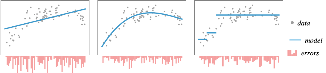
ModelFit fits and selects the best model from one or more candidates, returning a fitted model or a detailed report.
Model fitting can be used to predict values for unseen data, understand the relationships between variables, support decision-making and summarize patterns in complex datasets.

The value of a fitted model at a particular point {x₁,…} can be found using model[{x₁,…}].

Data

Possible forms of data are:

	{y₁,y₂,…}	equivalent to the form {{1,y₁},{2,y₂},…}
	{{x₁₁,x₁₂,…,y₁},…}	a list of independent values x_ij and the responses y_i
	{{x₁₁,x₁₂,…}y₁,…}	a list of rules between input values and responses
	{{x₁₁,x₁₂,…},…}{y₁,y₂,…}	a rule between a list of input values and responses
	{{x₁₁,…,y₁,…},…}n	fit the n column of a matrix
	Tabular[…]cspec	fit the columns cspec in a tabular object

The following forms of column specifications cspec are allowed for fitting tabular data:

	ycol	fit the response column ycol
	{xcol,ycol}	fit column ycol against column xcol
	{xcol₁,… ,ycol}	specify multiple predictor columns xcol_i
	{{xcol₁,…},ycol}	also specify multiple predictor columns xcol_i

Model

Possible model specifications include:
"name" fit a named model

model fit model on data

{model₁, model₂, …} fit all the model_i and select the best one
Named models include:
"Linear" PolynomialModel[1]

"Quadratic" PolynomialModel[2]

"Cubic" PolynomialModel[3]

"Exponential" ExponentialModel[]
Valid model specifications include:

	DecisionTreeModel[]	decision tree
	ExponentialModel[]	product of
	FormulaModel[expr,…]	generic expression expr
	LinearModel[basis,…]	linear combination of the terms in basis
	LogModel[]	sum of
	NearestModel[]	nearest neighbor model
	PerceptronModel[]	multilayer perceptron
	PeriodicModel[]	sum of
	PolynomialModel[d]	polynomial of degree d
	PowerModel[]	product of $alpha_i TemplateBox[{x, i, {beta, _, i}}, Subsuperscript]$

When specifying more then one model, ModelFit selects the best using cross validation. The best model is then trained on the full data.

Properties

Available properties props include:

	"Expression"	the model mathematical expression, when applicable
	"FittedModel"	a FittedModel object, when applicable
	"FittedModelList"	a list of FittedModel objects
	"Function"	the model as -ary pure function, when applicable
	"Model"	the best fitted model (default)
	"ModelList"	all the fitted models
	"ParameterAssociation"	association of parameter names and fitted values
	"ParameterRules"	list of parameter names and fitted values
	"Parameters"	fitted parameter values
	"Report"	a ModelFitReport object that can be queried
	"TabularFunction"	the model as function that applies on a row
	"Variables"	list of used variable names

Additionally, props can be any property of the models and the fit report.

Options

ModelFit takes the following options:

CriterionFunction	"RootMeanSquareError"	method of loss calcuation
RandomSeeding	1234	internal seeding of pseudorandom generators
ValidationSet	Automatic	data used to measure the trained models

The CriterionFunction option controls the function used to select the best model during cross validation.
In a regression task, the function is applied on the fit residuals r_i=y_i-.
In a classification task, the function compares a list of class probabilities {<|"class₁"p₁,…,|>,…} and a list of target classes {y₁,…}.
Possible settings for CriterionFunction include:

	"RootMeanSquaredError"	Sqrt[Mean[r^2]]
	"MeanSquaredError"	Mean[r^2]
	"MeanAbsoluteError"	Mean[Abs[r]]
	"MedianAbsoluteError"	Median[Abs[r]]
	"CrossEntropy"	-1/n Sum[Log[p〚i,y〚i〛〛],{i,n}]

Possible settings for RandomSeeding include:

	Automatic	automatically reseed every time the function is called
	Inherited	use externally seeded random numbers
	seed	use an explicit integer or strings as a seed

Possible settings for ValidationSet include:

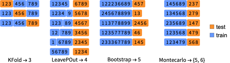
	Automatic	equivalent to "KFold"5
	"KFold"k	split data in k subsets, train on k-1
	"LeavePOut"p	test on p examples and train on the rest
	"LeaveOneOut"	equivalent to "LeavePOut"1
	"Montecarlo"{k,n}	random sampling k subsets without replacement
	"Bootstrap"k	random sampling k subsets with replacement
	Scaled[f]	use a fraction f of the input data

Examples

open all close all

Basic Examples (3)

Fit a polynomial expression to a list of values:

Wolfram Language code: ModelFit[{-4, -1, 4, 10, 20}, "Quadratic"]

Fit a regression line model to tabular data:

Wolfram Language code: ModelFit[ResourceData["Sample Data: Old Faithful Eruptions"], "Linear"]

Find the best fit among different models:

Wolfram Language code: ModelFit[ResourceData["Sample Data: Old Faithful Eruptions"], {PolynomialModel[], PowerModel[{0, a, b}, 1]}, "Report"]

Scope (18)

Data Specification (5)

Fit a list of values, assuming they are at integer spacing starting from one:

Wolfram Language code: ModelFit[{-4, -1, 4, 10, 20}, "Quadratic"]

Fit a list of points:

Wolfram Language code: ModelFit[{{1, -4}, {2, -1}, {3, 4}, {4, 10}, {5, 20}}, "Quadratic"]

Specify the data as a list of rules

Wolfram Language code: ModelFit[{1 -> -4, 2 -> -1, 3 -> 4, 4 -> 10, 5 -> 20}, "Quadratic"]

Fit the column of a matrix:

Wolfram Language code:

ModelFit[(⁠|      |     |      |
| ---- | --- | ---- |
| 1.3  | "P" | 1    |
| 1.8  | "Q" | 2.5  |
| 1.9  | "Q" | 3    |
| 0.2  | "P" | 1    |
| -3.2 | "P" | -4.2 |
| 0.3  | "Q" | 2    |⁠) -> 2, DecisionTreeModel[]]

Fit a tabular column:

Wolfram Language code:

data = Tabular[Association["RawSchema" -> Association["ColumnProperties" -> 
     Association["A" -> Association["ElementType" -> "Real64"], 
      "B" -> Association["ElementType" -> "Real64"]], "KeyColumns" -> None, 
    "Backend" -> "WolframKernel"], "Options" -> {AppearanceElements -> {"ColumnHeaders"}}, 
  "BackendData" -> Association["ColumnData" -> DataStructure["ColumnTable", 
      {{TabularColumn[Association["Data" -> {{0.7532169851483861, 0.04392850040375418, 
             -0.8275531460917351, -0.2441740913902284, -0.9767108540615066}, {}, None}, 
          "ElementType" -> "Real64"]], TabularColumn[Association[
          "Data" -> {{0.09726870121287412, -1.0066910140236667, 0.3732317268915213, 
             -0.7595363493288183, 0.9817034793118677}, {}, None}, "ElementType" -> "Real64"]]}}]]]];

Wolfram Language code: ModelFit[data -> "A", "Quadratic"]

By default, the final column is considered the response:

Wolfram Language code: ModelFit[data, "Quadratic"] == ModelFit[data -> "B", "Quadratic"]

Select both the input columns and the response:

Wolfram Language code: tabular = ResourceData["Sample Data: Fisher's Irises"];

Wolfram Language code: ModelFit[tabular -> {"PetalLength", "PetalWidth"}, "Linear"]

Specify multiple dependent variables:

Wolfram Language code: ModelFit[tabular -> {{"SepalLength", "SepalWidth"}, "PetalLength"}, "Linear"]

Model Specification (5)

Fit a specific model:

Wolfram Language code: ModelFit[{...}, PolynomialModel[2]]

Give explicit variable names:

Wolfram Language code: ModelFit[{...}, PolynomialModel[2, myvar], "Expression"]

Find the best model to fit the data:

Wolfram Language code: ModelFit[{...}, {PolynomialModel[2], ExponentialModel[]}]

Find the best model in a family:

Wolfram Language code: ModelFit[{...}, PolynomialModel[UpTo[4]]]

Use Span to specify the hyperparameter range:

Wolfram Language code: ModelFit[{...}, PolynomialModel[2 ;; 10 ;; 2]]

Specify a model with numerical parameter value:

Wolfram Language code: model = PolynomialModel[2, {5, a, b}, 1]

The parameter is considered fixed during fitting:

Wolfram Language code: ModelFit[{{0, 3}, {1, 4}, {2, 5}}, model]

Properties (8)

By default, the model is returned with the fitted parameters:

Wolfram Language code: ModelFit[{{1, 1}, {2, 4}, {2.5, 6}, {3, 9}}, PolynomialModel[2, {x}]]

This is the equivalent to the "Model" output:

Wolfram Language code: model = ModelFit[{{1, 1}, {2, 4}, {2.5, 6}, {3, 9}}, PolynomialModel[2, {x}], "Model"]

Get multiple properties from a fit:

Wolfram Language code: ModelFit[{{1, 1}, {2, 4}, {2.5, 6}, {3, 9}}, PolynomialModel[2, {x}], {"Model", "Function"}]

Use "Function" to get a variadic function:

Wolfram Language code: ModelFit[{{1, 1}, {2, 4}, {2.5, 6}, {3, 9}}, PolynomialModel[2, {x}], "Function"]

Use "TabularFunction" to get a function that works on a table row:

Wolfram Language code: ModelFit[{{1, 1}, {2, 4}, {2.5, 6}, {3, 9}}, PolynomialModel[2, {x}], "TabularFunction"]

Get a FittedModel object:

Wolfram Language code:

ModelFit[ResourceData["Sample Data: Fisher's Irises"] -> {"PetalLength", "PetalWidth"}, PolynomialModel[4], "FittedModel"]

Get a ModelFitReport for a single model:

Wolfram Language code: ModelFit[ResourceData["Sample Data: Old Faithful Eruptions"], PolynomialModel[4], "Report"]

Get a report for the cross-validation results and the best model found:

Wolfram Language code: report = ModelFit[ResourceData["Sample Data: Old Faithful Eruptions"], PolynomialModel[], "Report"]

Retrieve information from the report:

Wolfram Language code: report["CrossValidationChart"]

Get a list of the cross-validated models:

Wolfram Language code:

ModelFit[ResourceData["Sample Data: Fisher's Irises"] -> {"PetalLength", "PetalWidth"}, PolynomialModel[UpTo[5]], "ModelList"]

Options (5)

CriterionFunction (2)

Change the CriterionFunction to use a median absolute deviation:

Wolfram Language code: data = ResourceData["Sample Data: Old Faithful Eruptions"];

Wolfram Language code: medianModel = ModelFit[data, PolynomialModel[UpTo[3]], "FittedModel", CriterionFunction -> "MedianAbsoluteError" ]

Visualize the fit:

Wolfram Language code: ListPlot[ data, PlotFit -> medianModel]

Compare to result using the default "RootMeanSquaredError":

Wolfram Language code:

ListPlot[ data, PlotFit  -> ModelFit[data, PolynomialModel[UpTo[3]], "FittedModel", CriterionFunction -> "RootMeanSquaredError" ]]

Examine the ModelFitReport for comparison of model performance:

Wolfram Language code: report = ModelFit[{...}, PolynomialModel[], "Report", CriterionFunction -> "RootMeanSquaredError"]

Compare the losses of all input models on a single graph:

Wolfram Language code: report["CrossValidationChart"]

See a side-by-side comparison with a different method of loss calculation:

Wolfram Language code:

ModelFit[{...}, PolynomialModel[], "CrossValidationChart", CriterionFunction -> #]& /@ {"RootMeanSquaredError", "MedianAbsoluteError"}

ValidationSet (3)

Specify how the data is split during the cross validation:

Wolfram Language code:

ModelFit[ResourceData["Sample Data: Old Faithful Eruptions"], PolynomialModel[2 | 3 | 4], ValidationSet -> "LeavePOut" -> 10 ]

The default setting is "KFold"  5:

Wolfram Language code:

ModelFit[ResourceData["Sample Data: Old Faithful Eruptions"], PolynomialModel[2 | 3 | 4], ValidationSet -> "KFold" -> 5 ] === ModelFit[ResourceData["Sample Data: Old Faithful Eruptions"], PolynomialModel[2 | 3 | 4] ]

Small sets of data may suffer with the default K-fold of 5:

Wolfram Language code: data = {0.85, 0.3, 4.5, 2.91, 17.69, 25.9, 20.7, 20.11, 17.29, 5.54, 7.52, 7.72};

The default setting is keeping the model variance low:

Wolfram Language code: ListPlot[data, PlotFit -> PolynomialModel[UpTo[Length[data]]]]

Use a different validation setting to improve accuracy:

Wolfram Language code: ListPlot[data, PlotFit -> ModelFit[data, PolynomialModel[UpTo[Length[data]]], ValidationSet -> "LeaveOneOut"]]

Turning off validation typically results in a model that is overfitting the data:

Wolfram Language code: ListPlot[data, PlotFit -> ModelFit[data, PolynomialModel[UpTo[Length[data]]], ValidationSet -> None]]

The cross validation type is stated in the fit report:

Wolfram Language code: ModelFit[{...}, PolynomialModel[], "Report"]

Applications (1)

Brain to Body Size (1)

To compare brain sizes, retrieve data on the brain to body ratio:

Wolfram Language code: tab = ToTabular@ResourceData["Sample Data: Animal Weights"]

Inspect the data:

Wolfram Language code: plainData = Values@Normal@tab[[All, {"BodyWeight", "BrainWeight"}]] -> Normal@tab[[All, "Species"]];

Wolfram Language code: graph = ListLogLogPlot[plainData, LabelingFunction -> Tooltip, AxesLabel -> {"Body", "Brain"}]

Remove the three dinosaurs from the dataset:

Wolfram Language code: mammals = Discard[tab, MatchQ[#Species, "Triceratops" | "Diplodocus" | "Brachiosaurus"]&]

Due to the data range, use the logarithm of the data:

Wolfram Language code:

logMammal = ConstructColumns[mammals, {"Species", "LogBodyWeight" -> Function[Log[QuantityMagnitude[#BodyWeight]]], "LogBrainWeight" -> Function[Log[QuantityMagnitude[#BrainWeight]]]}]

Fit a linear model to the mammals:

Wolfram Language code: model = ModelFit[logMammal -> {"LogBodyWeight", "LogBrainWeight"}, "Linear"]

Compare the fit to the entire dataset (note the three outliers; these are the three dinosaurs):

Wolfram Language code:

Show[
	graph, 
	ListLogLogPlot[Table[{Exp[x], Exp[model[x]]}, {x, -4, 12}], Joined -> True, PlotHighlighting -> None]
	]

Properties & Relations (3)

Use the "FittedModel" property in the PlotFit option of ListPlot:

Wolfram Language code: ListPlot[{...}, PlotFit -> ModelFit[{...}, PowerModel[], "FittedModel"]]

Use Information to review details of a model after fitting:

Wolfram Language code: Information[ModelFit[{...}, PolynomialModel[2]]]

Retrieve specific properties:

Wolfram Language code: Information[ModelFit[{...}, PolynomialModel[2]], "Variables"]

Retrieve multiple properties simultaneously:

Wolfram Language code: Information[ModelFit[{...}, PolynomialModel[2]], {"Hyperparameters", "Parameters"}]

Static and initial values for parameters are typically determined by model specifications; for example, specify a PolynomialModel with a fixed intercept:

Wolfram Language code: ModelFit[{...}, PolynomialModel[2, {a -> 1, b, c}, 1]]

Use a PowerModel with an initial value for the power:

Wolfram Language code: ModelFit[{...}, PowerModel[{a, b, {c, -1}}, 1]]

Possible Issues (1)

Outliers or bad data can cause the fit to fail:

Wolfram Language code: data = ResourceData["Sample Data: Abalone Measurements"];

Attempt to fit a power law to the data:

Wolfram Language code: ModelFit[data -> {{"Diameter", "Height"}, "WholeWeight"}, PowerModel[]]

Inspect the data:

Wolfram Language code: ListPointPlot3D[data[[All, {"Diameter", "Height", "ShuckedWeight"}]], AxesLabel -> Automatic]

Discard the nonsensical -high crab from the dataset:

Wolfram Language code: cleanData = Discard[data, #["Height"] == Quantity[0, "Millimeters"]&];

Fit the model again:

Wolfram Language code: ModelFit[cleanData -> {{"Diameter", "Height"}, "WholeWeight"}, PowerModel[]]

Top

More Learning

Tech Support

Wolfram Solutions

Wolfram Solutions For Education

Get Started

Grow Your Skills

Work with Us

Educational Programs for Adults

Educational Programs for Youth

Read

ModelFit

Details and Options

Data

Model

Properties

Options

Examples

Basic Examples (3)

Scope (18)

Data Specification (5)

Model Specification (5)

Properties (8)

Options (5)

CriterionFunction (2)

ValidationSet (3)

Applications (1)

Brain to Body Size (1)

Properties & Relations (3)

Possible Issues (1)

Text

CMS

APA

BibTeX

BibLaTeX

	"Linear"	PolynomialModel[1]
	"Quadratic"	PolynomialModel[2]
	"Cubic"	PolynomialModel[3]
	"Exponential"	ExponentialModel[]

ModelFit

Details and Options

Data

Model

Properties

Options

Examples

Basic Examples (3)

Scope (18)

Data Specification (5)

Model Specification (5)

Properties (8)

Options (5)

CriterionFunction (2)

ValidationSet (3)

Applications (1)

Brain to Body Size (1)

Properties & Relations (3)

Possible Issues (1)

See Also

Related Guides

History

Text

CMS

APA

BibTeX

BibLaTeX