Wolfram Language & System Documentation Center

RStabilityConditions[eqn,a[n],n]

gives the fixed points and stability conditions for a recurrence equation.

RStabilityConditions[{eqn₁,eqn₂,…},{a₁[n],a₂[n],…},n]

gives the fixed points and stability conditions for a system of recurrence equations.

RStabilityConditions[{eqn₁,eqn₂,…},{a₁[n],a₂[n],…},n,{pnt₁,pnt₂,…}]

gives stability conditions only for the given fixed points.

RStabilityConditions

RStabilityConditions[eqn,a[n],n]

gives the fixed points and stability conditions for a recurrence equation.

RStabilityConditions[{eqn₁,eqn₂,…},{a₁[n],a₂[n],…},n]

gives the fixed points and stability conditions for a system of recurrence equations.

RStabilityConditions[{eqn₁,eqn₂,…},{a₁[n],a₂[n],…},n,{pnt₁,pnt₂,…}]

gives stability conditions only for the given fixed points.

Details and Options

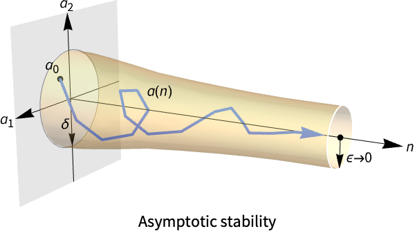
Stability is also known as asymptotic stability and fixed points are also known as equilibrium points or stationary points.
RStabilityConditions is typically used to qualitatively analyze long-term behavior near fixed points. If the system is stable, then solutions converge to the fixed point if you are close enough.
For a system of recurrence equations , a point is a fixed point iff . In effect, the initial value remains stationary; if you initialize at you stay at .
A fixed point is asymptotically stable iff for and you have $TemplateBox[{{a, (, n, )}, n, infty}, Limit2Arg]=a^*$ for sufficiently small.

RStabilityConditions returns a list of the form {{{,,…},cond},…}, where {,,…} is a fixed point.
RStabilityConditions gives sufficient conditions for local stability of fixed points. For linear systems, these conditions are also conditions for global stability.
RStabilityConditions works for linear and nonlinear ordinary difference equations.
The following options can be given:
Assumptions $Assumptions assumptions on parameters

Examples

open all close all

Basic Examples (5)

Find the fixed point and determine its stability for the recursion :

Wolfram Language code: RStabilityConditions[a[n + 1] == (1/2)a[n], a[n], n]

Find the fixed point and determine the stability for the recursion :

Wolfram Language code: RStabilityConditions[a[n + 1] == 2a[n] + 1, a[n], n]

Find the fixed points and conditions for stability for the recursion :

Wolfram Language code: RStabilityConditions[y[n + 1] == a y[n], y, n]

Plot several solutions for different values of a:

Wolfram Language code: sol = RSolveValue[{y[n + 1] == a y[n], y[0] == 1}, y[n], n]

Wolfram Language code: Table[DiscretePlot[sol, {n, 0, 20}, ...], {a, {-1.1, 0.8, 1.1}}]

Stability analysis of a two-dimensional system:

Wolfram Language code: RStabilityConditions[{x[1 + n] == b x[n] + y[n], y[1 + n] == -2 x[n] + a y[n]}, {x, y}, n]

Plot the parameter region for which the system is stable:

Wolfram Language code: RegionPlot[%[[1, 2]], {a, -3, 3}, {b, -3, 3}]

Find the fixed points for a nonlinear system of three ODEs:

Wolfram Language code:

sys = {x[n + 1] == (x[n] + 3 y[n]/4 + x[n] + y[n] + z[n]), y[n + 1] == (y[n] + 2 z[n]/4 + x[n] + y[n] + z[n]), z[n + 1] == (z[n]/4 + x[n] + y[n] + z[n])};

Wolfram Language code: points = RFixedPoints[sys, {x[n], y[n], z[n]}, n]

Study the stability of the first point:

Wolfram Language code: RStabilityConditions[sys, {x[n], y[n], z[n]}, n, {{-3, 0, 0}}]

Study the stability of the second point:

Wolfram Language code: RStabilityConditions[sys, {x[n], y[n], z[n]}, n, {{0, 0, 0}}]

Scope (15)

Linear Equations (4)

Find the fixed point and determine its stability for the recursion :

Wolfram Language code: RStabilityConditions[a[n + 1] == 1 / 3 a[n], a[n], n]

A first-order linear inhomogeneous equation:

Wolfram Language code: RStabilityConditions[y[n + 1] == a y[n] + 5, y, n]

Plot the solution for :

Wolfram Language code:

sol = RSolveValue[{y[n + 1] == a y[n] + 5, y[0] == 1}, y[n], n];
DiscretePlot[sol /. a -> 0.5, {n, 0, 20}]

Plot the solution for :

Wolfram Language code:

sol = RSolveValue[{y[n + 1] == a y[n] + 5, y[0] == 1}, y[n], n];
DiscretePlot[sol /. a -> 1.5, {n, 0, 20}]

Second-order linear equation:

Wolfram Language code: RStabilityConditions[y[n + 2] + a y[n + 1] + b y[n] == 0, y, n]

Plot the stability region:

Wolfram Language code: RegionPlot[%[[1, 2]], {a, -2, 2}, {b, -2, 2}, FrameLabel -> {a, b}]

Third-order linear equation:

Wolfram Language code: RStabilityConditions[y[n + 3] + a y[n + 2] + b y[n + 1] + c y[n] == 0, y, n]

Plot the stability region:

Wolfram Language code: RegionPlot3D[%[[1, 2]], {b, -2, 2}, {c, -2, 2}, {a, -2, 2}, ...]

Nonlinear Equations (4)

Stability analysis of a nonlinear recurrence equation:

Wolfram Language code: RStabilityConditions[x[n + 1] == x[n]^2 + 3x[n], x, n]

Use a cobweb plot to demonstrate the stability:

Wolfram Language code: ResourceFunction["CobwebPlot"][x |-> x^2 + 3x, -2.9, 10, {-3, 1}, Rule[...]]

The stability of a logistic equation:

Wolfram Language code: RStabilityConditions[a[n + 1] == 2(1 - a[n])a[n], a[n], n]

Plot the solution:

Wolfram Language code: sol = Quiet[RSolveValue[{a[n + 1] == 2(1 - a[n])a[n], a[0] == 1 / 10}, a[n], n]]

Wolfram Language code: DiscretePlot[%, {n, 0, 20}]

Use a cobweb plot to demonstrate the stability:

Wolfram Language code: ResourceFunction["CobwebPlot"][a |-> 2(1 - a)a, 0.1, 10, {-0.2, 0.8}]

The stability of a Riccati equation:

Wolfram Language code: RStabilityConditions[a[n + 1] == -(a[n] + 15) / (a[n] + 7), a[n], n]

Use a cobweb plot to demonstrate the stability:

Wolfram Language code: ResourceFunction["CobwebPlot"][a |-> -(a + 15) / (a + 7), -4.5, 10, {-5.3, 0}]

Higher-order equations:

Wolfram Language code: RStabilityConditions[ a[n + 2] == a[n + 1] a[n] ^ 2, a[n], n]

Wolfram Language code: RStabilityConditions[ a[n + 2] == b ^ n a[n + 1] a[n] ^ 2, a[n], n]

Linear Systems (5)

The stability of a linear system of uncoupled equations:

Wolfram Language code: RStabilityConditions[{x[n + 1] == 1 / 2x[n], y[n + 1] == 1 / 3y[n]}, {x, y}, n]

The stability of a linear system with constant coefficients:

Wolfram Language code: RStabilityConditions[{y[n + 1] == 3 - z[n], z[n + 1] == (1 - y[n]/2)}, {y[n], z[n]}, n]

Use VectorPlot to visualize the stability:

Wolfram Language code: VectorPlot[{3 - z - y, (1 - y/2) - z}, {y, 3, 7}, {z, -5, 2}, Rule[...]]

Solve the system with boundary conditions:

Wolfram Language code: sol = RSolve[{y[n + 1] + z[n] == 3, y[n] + 2 z[n + 1] == 1, y[0] == 4, z[0] == 1}, {y, z}, n]

Plot the solution:

Wolfram Language code: DiscretePlot[Evaluate[{y[n], z[n]} /. sol[[1]]], {n, 0, 20}]

A first-order system with periodic coefficients:

Wolfram Language code: RStabilityConditions[{x[n + 1] == (1 / 2) * (2 + (-1) ^ n)y[n], y[n + 1] == (1 / 2)(2 - (-1) ^ n) * x[n]}, {x, y}, n]

Compare with the general solution:

Wolfram Language code: sol = RSolve[{x[n + 1] == (1 / 2) * (2 + (-1) ^ n)y[n], y[n + 1] == (1 / 2)(2 - (-1) ^ n) * x[n]}, {x, y}, n]

Wolfram Language code: DiscretePlot[Evaluate[{x[n], y[n]} /. sol[[1]] /. {C[1] -> 1, C[2] -> 2}], {n, 0, 20}]

A first-order system with eventually periodic coefficients:

Wolfram Language code: RStabilityConditions[{x[n + 1] == Mod[2 ^ n, 6]y[n], y[n + 1] == (1 / 2) * (2 - (-1) ^ n) * x[n]}, {x, y}, n]

Analyze the stability of a 10x10 discrete linear system with random constant coefficients:

Wolfram Language code:

SeedRandom[1234];
m = RandomInteger[10, {10, 10}];
g = RandomInteger[10, 10];

Wolfram Language code: dep = {x1[n], x2[n], x3[n], x4[n], x5[n], x6[n], x7[n], x8[n], x9[n], x10[n]};

Wolfram Language code: sys = Thread[(dep /. n -> n + 1) == m.dep + g];

Wolfram Language code: RStabilityConditions[sys, dep, n]

Nonlinear Systems (2)

A nonlinear first-order system:

Wolfram Language code:

RStabilityConditions[{x1[n + 1] == x1[n] - x2[n](1 - x2[n]), x2[n + 1] == x1[n] / 13, x3[n + 1] == x3[n] / 2 + x1[n]}, 
  {x1, x2, x3}, n]

Check only the stability of the first fixed point:

Wolfram Language code:

RStabilityConditions[{x1[n + 1] == x1[n] - x2[n](1 - x2[n]), x2[n + 1] == x1[n] / 13, x3[n + 1] == x3[n] / 2 + x1[n]}, 
  {x1, x2, x3}, n, {{0, 0, 0}}]

Check only the stability of the second fixed point:

Wolfram Language code:

RStabilityConditions[{x1[n + 1] == x1[n] - x2[n](1 - x2[n]), x2[n + 1] == x1[n] / 13, x3[n + 1] == x3[n] / 2 + x1[n]}, 
  {x1, x2, x3}, n, {{13, 1, 26}}]

The stability of a linear fractional system:

Wolfram Language code: RStabilityConditions[{y[n + 1] == (3y[n]/1 + y[n] + z[n]), z[n + 1] == (z[n]/1 + y[n] + z[n])}, {y[n], z[n]}, n]

Use VectorPlot to visualize the stability at point :

Wolfram Language code: VectorPlot[{(3y/1 + y + z) - y, (z/1 + y + z) - z}, {y, -2, 4}, {z, -2, 2}, Rule[...]]

Options (1)

Assumptions (1)

Without Assumptions, there are conditions on parameters for stability:

Wolfram Language code: RStabilityConditions[y[n + 1] == a y[n], y, n]

Using Assumptions can often result in simplified conditions:

Wolfram Language code: RStabilityConditions[y[n + 1] == a y[n], y, n, Assumptions -> 0 < a < 1 / 2]

Applications (8)

Numerical Analyses (3)

Analyze the stability of the Newton–Raphson difference equation for the function x²-a:

Wolfram Language code: f[x_] := x^2 - a

The recurrence equation for the method is:

Wolfram Language code: eqn = x[n + 1] == x[n] - (f[x[n]]/D[f[x[n]], x[n]])

Study the stability of the system:

Wolfram Language code: RStabilityConditions[eqn, x, n]

Visualize the stability of fixed points for :

Wolfram Language code:

pl1 = ResourceFunction["CobwebPlot"][x |-> x - (-4 + x^2/2 x), 1, 10, {0, 3}];
pl2 = ResourceFunction["CobwebPlot"][x |-> x - (-4 + x^2/2 x), -1, 10, {-3, 0}];
Show[pl1, pl2, PlotRange -> All]

Analyze the stability of the Newton–Raphson difference equation for the function x^1/3:

Wolfram Language code: f[x_] := x^1 / 3

The recurrence equation for the method is:

Wolfram Language code: eqn = x[n + 1] == x[n] - (f[x[n]]/D[f[x[n]], x[n]])

The equation has one unstable fixed point at origin:

Wolfram Language code: RStabilityConditions[eqn, x, n]

The instability of the point means that Newton's method cannot be used in this case:

Wolfram Language code: x1[n_] = RSolveValue[{eqn, x[0] == 1}, x[n], n]

Wolfram Language code: TableForm[Quiet[Table[{x1[n], N[Abs[f[x1[n]]]]}, {n, 0, 10}]], TableHeadings -> {None, {"x[n]", "f[x[n]]"}}]

Consider a system of linear equations , where:

Wolfram Language code:

A = {{16, 3}, {7, -11}};
b = {11, 13};

Construct the Gauss–Seidel difference equation for the system:

Wolfram Language code: L = LowerTriangularize[A];

Wolfram Language code: U = UpperTriangularize[A, 1];

Wolfram Language code: reqn = Thread[{x1[n + 1], x2[n + 1]} == Inverse[L].(b - U.{x1[n], x2[n]})]

Analyze the stability of the Gauss–Seidel equation:

Wolfram Language code: RStabilityConditions[reqn, {x1, x2}, n]

Solve the system using LinearSolve:

Wolfram Language code: LinearSolve[A, b]

Physics (1)

Consider an object with temperature in the environment with constant temperature . Let be the change in temperature of the object over a time interval . Newton's law of cooling states that the rate of change of the temperature of an object is proportional to the difference of the temperature of the object and its surroundings:

Wolfram Language code: eqn = t[n + 1] == t[n] + k(r - t[n]);

The equation is stable if :

Wolfram Language code: RStabilityConditions[eqn, t, n]

Solution of the equation:

Wolfram Language code: sol = RSolveValue[{eqn, t[0] == t0}, t[n], n]

Simulate the cooling process:

Wolfram Language code: DiscretePlot[Evaluate[sol /. {r -> 20, t0 -> 40, k -> 1 / 2}], {n, 0, 10}]

Simulate the heating process:

Wolfram Language code: DiscretePlot[Evaluate[sol /. {r -> 20, t0 -> 10, k -> 1 / 2}], {n, 0, 10}]

Ecology and Biology (2)

Stability analysis for the competing species model:

Wolfram Language code: RStabilityConditions[{a[n + 1] == 1.047a[n] - 0.012a[n]b[n], b[n + 1] == 1.023b[n] - 0.015a[n]b[n]}, {a, b}, n]

Solve the equation for given initial conditions and plot the solution:

Wolfram Language code:

sol = RecurrenceTable[{a[n + 1] == 1.047a[n] - 0.012a[n]b[n], b[n + 1] == 1.023b[n] - 0.015a[n]b[n], a[0] == 25, b[0] == 30}, {a[n], b[n]}, {n, 0, 50}];

Wolfram Language code: ListPlot[{#[[1]]& /@ sol, #[[2]]& /@ sol}, PlotLegends -> {a[n], b[n]}]

Stability analysis for the predator-prey model:

Wolfram Language code: RStabilityConditions[{a[n + 1] == 0.99a[n] + 0.0001a[n]b[n], b[n + 1] == 1.1b[n] - 0.0005a[n]b[n]}, {a, b}, n]

Vector field plot of the model:

Wolfram Language code: VectorPlot[{0.99a + 0.0001a b - a, 1.1b - 0.0005a b - b}, {a, 0, 300}, {b, 0, 300}]

Solve the system and plot solutions:

Wolfram Language code:

sol = RecurrenceTable[{a[n + 1] == 0.99a[n] + 0.0001a[n]b[n], b[n + 1] == 1.1b[n] - 0.0005a[n]b[n], a[0] == 25, b[0] == 100}, {a[n], b[n]}, {n, 0, 1000}];

Wolfram Language code: ListPlot[{#[[1]]& /@ sol, #[[2]]& /@ sol}, PlotLegends -> {"Predator", "Prey"}, PlotRange -> All]

Economics (2)

Consider a bank account with initial deposit , annual rate and monthly withdrawal amount . The amount in the saving account after months satisfies a recurrence equation:

Wolfram Language code: eqn = a[n + 1] == (1 + (r/1200))a[n] - v;

The equation has an unstable fixed point :

Wolfram Language code: RStabilityConditions[a[n + 1] == (1 + (r/1200))a[n] - v, a, n, Assumptions -> 0 <= r < 100]

The amount in the account will increase each month if :

Wolfram Language code: sol1 = RSolveValue[{a[n + 1] == (1 + (r/1200))a[n] - v, a[0] == (1201 v/r)}, a[n], n];

Wolfram Language code: sol2 = RSolveValue[{a[n + 1] == (1 + (r/1200))a[n] - v, a[0] == (1199 v/r)}, a[n], n];

Wolfram Language code: DiscretePlot[Evaluate[{sol1, sol2} /. {v -> 1000, r -> 6}], {n, 0, 50}]

Stability analysis for the logistic equation:

Wolfram Language code: RFixedPoints[y[n + 1] == r y[n](1 - y[n]), y, n]

Check the stability of the fixed points:

Wolfram Language code: RStabilityConditions[y[n + 1] == r y[n](1 - y[n]), y, n]

Check the stability for given range of the parameter :

Wolfram Language code: RStabilityConditions[y[n + 1] == r y[n](1 - y[n]), y, n, Assumptions -> 1 < r < 3]

Visualize the stability for :

Wolfram Language code: ResourceFunction["CobwebPlot"][y |-> r y(1 - y) /. r -> 1 / 2, 0.8, 10, {-1, 1}]

Visualize the stability for :

Wolfram Language code: ResourceFunction["CobwebPlot"][y |-> r y(1 - y) /. r -> 2, 0.8, 10, {-1, 1}, PlotRange -> {-1, 1}]

Properties & Relations (9)

RStabilityConditions returns fixed points and stability conditions for recurrence equations:

Wolfram Language code: RStabilityConditions[y[n + 1] == a y[n], y, n]

Wolfram Language code: RStabilityConditions[a[n + 1] == (1/2)a[n], a[n], n]

Wolfram Language code: RStabilityConditions[y[n + 1] == 2 y[n], y, n]

Use RFixedPoints to find all fixed points of a recurrence equation:

Wolfram Language code: RFixedPoints[y[n + 1] == 2 y[n](1 - y[n]), y[n], n]

Analyze the stability at specific fixed points:

Wolfram Language code: RStabilityConditions[y[n + 1] == 2 y[n](1 - y[n]), y[n], n, {{0}}]

Wolfram Language code: RStabilityConditions[y[n + 1] == 2 y[n](1 - y[n]), y[n], n, {{1 / 2}}]

Use RFixedPoints to find all fixed points of a nonlinear recurrence equation:

Wolfram Language code: points = RFixedPoints[x[n + 1] == x[n]^2 + 3x[n], x, n]

Use Solve to find the fixed points:

Wolfram Language code: Solve[x^2 + 3x == x, x]

Linearize the equation near the first fixed point:

Wolfram Language code:

f1 = D[x^2 + 3x, x] /. x -> points[[1, 1]];
leqn1 = x[n + 1] == f1 x[n]

Check the stability near the first fixed point:

Wolfram Language code: RStabilityConditions[leqn1, x, n][[1, 2]]

Linearize the equation near the second fixed point:

Wolfram Language code:

f1 = D[x^2 + 3x, x] /. x -> points[[2, 1]];
leqn2 = x[n + 1] == f1 x[n]

Check the stability near the second fixed point:

Wolfram Language code: RStabilityConditions[leqn2, x, n][[1, 2]]

Determine the stability of the nonlinear equation using RStabilityConditions:

Wolfram Language code: RStabilityConditions[x[n + 1] == x[n]^2 + 3x[n], x, n]

The fixed points for an n-order recurrence equation are n-dimensional vectors:

Wolfram Language code: RStabilityConditions[y[n + 2] + y[n + 1] + 3 y[n] == 5, y, n]

The fixed points for a system of n first-order recurrence equations are n-dimensional vectors:

Wolfram Language code: RStabilityConditions[{y[n + 1] + z[n] == 3, y[n] + 2 z[n + 1] == 1}, {y[n], z[n]}, n]

Consider a system , :

Wolfram Language code:

f1[y1_, y2_] := 3y1 - y2;
f2[y1_, y2_] := (1 - y1 + y2/2);

Wolfram Language code: RStabilityConditions[{y1[n + 1] == f1[y1[n], y2[n]], y2[n + 1] == f2[y1[n], y2[n]]}, {y1[n], y2[n]}, n]

Calculate the differences and to generate the vector field plot of the system:

Wolfram Language code: VectorPlot[{f1[y1, y2] - y1, f2[y1, y2] - y2}, {y1, -2, 2}, {y2, -2, 2}, Rule[...]]

Analyze the stability of a system of two ODEs:

Wolfram Language code: RStabilityConditions[{a[n + 1] - b[n] == 2, a[n] - 3 b[n + 1] == 5}, {a, b}, n]

Use RSolveValue to solve the system using a fixed point as initial condition:

Wolfram Language code: sol = RSolveValue[{a[n + 1] - b[n] == 2, a[n] - 3 b[n + 1] == 5, a[0] == 1 / 2, b[0] == -3 / 2}, {a[n], b[n]}, n]

Use RSolveValue to solve the system for given initial conditions:

Wolfram Language code: sol = RSolveValue[{a[n + 1] - b[n] == 2, a[n] - 3 b[n + 1] == 5, a[0] == 3, b[0] == 1}, {a[n], b[n]}, n]

Plot the solution:

Wolfram Language code: DiscretePlot[Evaluate[sol], {n, 0, 20}]

Analyze the stability of a nonlinear ODE:

Wolfram Language code: RStabilityConditions[x[n + 1] == (1/2)x[n](1 - x[n]), x, n]

Solve the ODE using RecurrenceTable:

Wolfram Language code: sol = RecurrenceTable[{x[n + 1] == (1/2)x[n](1 - x[n]), x[0] == -9 / 10}, x, {n, 0, 20}, WorkingPrecision -> 10]

Plot the solution:

Wolfram Language code: ListPlot[sol, PlotRange -> All]

Analyze the stability of a recurrence equation with eventually constant coefficients:

Wolfram Language code: RStabilityConditions[y[n + 1] == ((1 / 2n ^ 3 + 1) / n ^ 3)y[n], y, n]

Find a series solution using AsymptoticRSolveValue:

Wolfram Language code: asol = AsymptoticRSolveValue[{y[n + 1] == ((1 / 2n ^ 3 + 1) / n ^ 3)y[n]}, y[n], {n, ∞, 10}]

Plot the asymptotic solution:

Wolfram Language code: DiscretePlot[asol /. {C[1] -> -0.1}, {n, 2, 30}, PlotRange -> All]

Possible Issues (2)

Sometimes the conditions for stability are not the simplest possible:

Wolfram Language code: RStabilityConditions[y[n + 1] == r y[n](a - y[n]), y, n, Assumptions -> Re[a] == 0]

Additional simplification can be achieved by further processing:

Wolfram Language code: Reduce[%[[1, 2]] && Re[a] == 0]

RStabilityConditions fails because the given point is not a fixed point:

Wolfram Language code: RStabilityConditions[y[n + 1] == y[n](1 - y[n]), y, n, {{1}}]

Use RFixedPoints to find all fixed points of the equation first:

Wolfram Language code: points = RFixedPoints[y[n + 1] == 3 y[n](1 - y[n]), y[n], n]

Wolfram Language code: RStabilityConditions[y[n + 1] == 3 y[n](1 - y[n]), y, n, {points[[1]]}]

Wolfram Language code: RStabilityConditions[y[n + 1] == 3 y[n](1 - y[n]), y, n, {points[[2]]}]

Top

More Learning

Tech Support

Wolfram Solutions

Wolfram Solutions For Education

Get Started

Grow Your Skills

Work with Us

Educational Programs for Adults

Educational Programs for Youth

Read

RStabilityConditions

Details and Options

Examples

Basic Examples (5)

Scope (15)

Linear Equations (4)

Nonlinear Equations (4)

Linear Systems (5)

Nonlinear Systems (2)

Options (1)

Assumptions (1)

Applications (8)

Numerical Analyses (3)

Physics (1)

Ecology and Biology (2)

Economics (2)

Properties & Relations (9)

Possible Issues (2)

Text

CMS

APA

BibTeX

BibLaTeX

RStabilityConditions

Details and Options

Examples

Basic Examples (5)

Scope (15)

Linear Equations (4)

Nonlinear Equations (4)

Linear Systems (5)

Nonlinear Systems (2)

Options (1)

Assumptions (1)

Applications (8)

Numerical Analyses (3)

Physics (1)

Ecology and Biology (2)

Economics (2)

Properties & Relations (9)

Possible Issues (2)

See Also

Related Guides

History

Text

CMS

APA

BibTeX

BibLaTeX