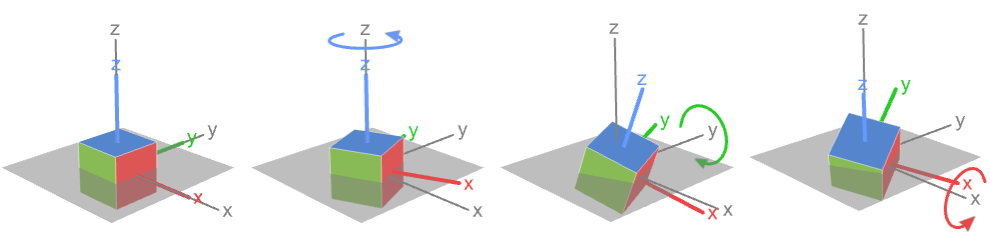
RollPitchYawMatrix[{α,β,γ}]
gives the 3D rotation matrix formed by rotating by α around the initial ![]() axis, then by β around the initial
axis, then by β around the initial ![]() axis, and then by γ around the initial
axis, and then by γ around the initial ![]() axis.
axis.


RollPitchYawMatrix
RollPitchYawMatrix[{α,β,γ}]
gives the 3D rotation matrix formed by rotating by α around the initial ![]() axis, then by β around the initial
axis, then by β around the initial ![]() axis, and then by γ around the initial
axis, and then by γ around the initial ![]() axis.
axis.
RollPitchYawMatrix[{α,β,γ},{a,b,c}]
gives the 3D rotation matrix formed by rotating by α around the fixed a axis, then by β around the fixed b axis, and then by γ around the fixed c axis.
Details and Options
- RollPitchYawMatrix is also known as bank-elevation-heading matrix or Cardan matrix. The angles {α,β,γ} are often referred to as Cardan angles, Tait–Bryan angles, nautical angles, bank-elevation-heading, or roll-pitch-yaw.
- RollPitchYawMatrix is typically used to specify a rotation as a sequence of basic rotations around coordinate axes where each rotation is referring to the initial or extrinsic coordinate frame.
- RollPitchYawMatrix[{α,β,γ}] is equivalent to RollPitchYawMatrix[{α,β,γ},{3,2,1}].
- RollPitchYawMatrix[{α,β,γ},{a,b,c}] is equivalent to
 where Rα,a=RotationMatrix[α,UnitVector[3,a]] etc.
 - The default z-y-x rotation RollPitchYawMatrix[{α,β,γ},{3,2,1}]:
- The rotation axes a, b, and c can be any integer 1, 2, or 3, but there are only twelve combinations that are general enough to be able to specify any 3D rotation.
- Rotations with the first and last axis repeated:
-
{3,2,3} z-y-z rotation 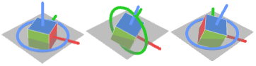
{3,1,3} z-x-z rotation 
{2,3,2} y-z-y rotation 
{2,1,2} y-x-y rotation 
{1,3,1} x-z-x rotation 
{1,2,1} x-y-x rotation 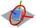
- Rotations with all three axes different:
-
{1,2,3} x-y-z rotation 
{1,3,2} x-z-y rotation 
{2,1,3} y-x-z rotation 
{2,3,1} y-z-x rotation 
{3,1,2} z-x-y rotation 
{3,2,1} z-y-x rotation (default) 
- Rotations with subsequent axes repeated still produce a rotation matrix, but cannot be inverted uniquely using RollPitchYawAngles.
- RollPitchYawMatrix supports the option TargetStructure, which specifies the structure of the returned matrix. Possible settings for TargetStructure include:
-
Automatic automatically choose the representation returned "Dense" represent the matrix as a dense matrix "Orthogonal" represent the matrix as an orthogonal matrix "Unitary" represent the matrix as a unitary matrix - RollPitchYawMatrix[…,TargetStructureAutomatic] is equivalent to RollPitchYawMatrix[…,TargetStructure"Dense"].
Examples
open all close allBasic Examples (2)
The standard roll-pitch-yaw matrix:
RollPitchYawMatrix[{α, β, γ}] /. {Cos[x_] :> Subscript[c, x], Sin[x_] :> Subscript[s, x]}//MatrixFormRotate an axes-aligned unit cube:
m = RollPitchYawMatrix[{(π/4), (π/3), (3π/4)}];Graphics3D[GeometricTransformation[Cuboid[], m]]Scope (5)
Give the standard z-y-x roll-pitch-yaw rotation matrix with ![]() ,
, ![]() , and
, and ![]() :
:
(m = RollPitchYawMatrix[{(3π/4), (π/3), (π/3)}])//MatrixFormv1 = {1, 0, 0};
v2 = m.v1Visualize the rotated vector (red):
Graphics3D[{Arrow[{{0, 0, 0}, v1}], Red, Arrow[{{0, 0, 0}, v2}]}]Give an x-y-z roll-pitch-yaw rotation matrix by specifying the second argument:
m = RollPitchYawMatrix[{(3π/4), (π/3), (π/3.)}, {1, 2, 3}]Rotate and visualize the vector {1,0,0}:
v1 = {1, 0, 0}; v2 = m.v1;Graphics3D[{Arrow[{{0, 0, 0}, v1}], Red, Arrow[{{0, 0, 0}, v2}]}]Rotate primitives in 3D graphics using GeometricTransformation:
m = RollPitchYawMatrix[{(π/4), (π/3), (3π/4)}];before = {Blue, Cuboid[], Green, Point[{1, 1, 1}]};
after = {Red, GeometricTransformation[Cuboid[], m], Green, GeometricTransformation[Point[{1, 1, 1}], m]};Graphics3D[{PointSize[.05], before, after}]Rotate a region using TransformedRegion:
s1 = [image];m = RollPitchYawMatrix[{Pi / 4, -Pi / 2, -Pi / 4}];s2 = TransformedRegion[s1, AffineTransform@m];{s1, s2}Rotate a 3D image using ImageTransformation:
r1 = ExampleData[{"TestImage3D", "Orbits"}];m = RollPitchYawMatrix[{Pi / 4, -Pi / 4, -Pi / 4}];r2 = ImageTransformation[r1, InverseFunction@AffineTransform@m, PlotRange -> All];{r1, r2}Options (1)
TargetStructure (1)
Return the roll-pitch-yaw rotation matrix as a dense matrix:
RollPitchYawMatrix[{(3π/4), (π/3), (π/3)}, TargetStructure -> "Dense"]Return the roll-pitch-yaw rotation matrix as an orthogonal matrix:
RollPitchYawMatrix[{(3π/4), (π/3), (π/3)}, TargetStructure -> "Orthogonal"]Return the roll-pitch-yaw rotation matrix as a unitary matrix:
RollPitchYawMatrix[{(3π/4), (π/3), (π/3)}, TargetStructure -> "Unitary"]Applications (6)
Illustrations (1)
Build a function that illustrates Euler rotations, showing the axis that is being rotated around:
$scene = First@[image];RollPitchYawRotationIllustration[{α_, β_, γ_}, {a_, b_, c_}] :=
Map[Graphics3D[GeometricTransformation[$scene, #], PlotRange -> 1.2, ImageSize -> 110, BoxStyle -> LightGray]&,
{RollPitchYawMatrix[{0, 0, 0}, {a, b, c}], RollPitchYawMatrix[{α, 0, 0}, {a, b, c}], RollPitchYawMatrix[{α, β, 0}, {a, b, c}], RollPitchYawMatrix[{α, β, γ}, {a, b, c}]}
]Here are all six of the a-b-c axes rotations. First is the standard z-y-x roll-pitch-yaw rotation:
RollPitchYawRotationIllustration[{Pi / 2, Pi / 2, Pi / 2}, {3, 2, 1}]The x-y-z roll-pitch-yaw rotation:
RollPitchYawRotationIllustration[{Pi / 2, Pi / 2, Pi / 2}, {1, 2, 3}]The x-z-y roll-pitch-yaw rotation:
RollPitchYawRotationIllustration[{Pi / 2, Pi / 2, Pi / 2}, {1, 3, 2}]The y-x-z roll-pitch-yaw rotation:
RollPitchYawRotationIllustration[{Pi / 2, Pi / 2, Pi / 2}, {2, 1, 3}]The y-z-x roll-pitch-yaw rotation:
RollPitchYawRotationIllustration[{Pi / 2, Pi / 2, Pi / 2}, {2, 3, 1}]The z-x-y roll-pitch-yaw rotation:
RollPitchYawRotationIllustration[{Pi / 2, Pi / 2, Pi / 2}, {3, 1, 2}]Then there are the six a-b-a axes rotations. First is the x-y-x roll-pitch-yaw rotation:
RollPitchYawRotationIllustration[{Pi / 2, Pi / 2, Pi / 2}, {1, 2, 1}]The x-z-x roll-pitch-yaw rotation:
RollPitchYawRotationIllustration[{Pi / 2, Pi / 2, Pi / 2}, {1, 3, 1}]The y-x-y roll-pitch-yaw rotation:
RollPitchYawRotationIllustration[{Pi / 2, Pi / 2, Pi / 2}, {2, 1, 2}]The y-z-y roll-pitch-yaw rotation:
RollPitchYawRotationIllustration[{Pi / 2, Pi / 2, Pi / 2}, {2, 3, 2}]The z-x-z roll-pitch-yaw rotation:
RollPitchYawRotationIllustration[{Pi / 2, Pi / 2, Pi / 2}, {3, 1, 3}]The z-y-z roll-pitch-yaw rotation:
RollPitchYawRotationIllustration[{Pi / 2, Pi / 2, Pi / 2}, {3, 2, 3}]Gimbal (5)
A gimbal is a system of pivoted rings that allows an object to orient itself in an arbitrary direction. These are used in various navigations and imaging applications:
ring3 = {Red, CapForm -> None, Tube[{{-.1, 0, 0}, {.1, 0, 0}}, 3], Line[{{{0, 0, 4}, {0, 0, 3}}, -{{0, 0, 4}, {0, 0, 3}}}]};
ring2 = {Blue, CapForm -> None, Tube[{{-.1, 0, 0}, {.1, 0, 0}}, 2], Line[{{{0, 3, 0}, {0, 2, 0}}, -{{0, 3, 0}, {0, 2, 0}}}]};
ring1 = {Green, CapForm -> None, Tube[{{-.1, 0, 0}, {.1, 0, 0}}, 1], Line[{{{0, 0, 1}, {0, 0, 2}}, -{{0, 0, 1}, {0, 0, 2}}}], Orange, Arrow[{{-1, 0, 0}, {1, 0, 0}}]};
The orientation of the object within a gimbal can be modeled using RollPitchYawMatrix with the angles of the rings' rotations, from the outermost to the innermost rings. Note that an a-b-a axis system is used:
gimbal[{α_, β_, γ_}] := With[{},
	Graphics3D[{GeometricTransformation[ring3, RollPitchYawMatrix[{0, 0, γ}, {3, 2, 3}]], GeometricTransformation[ring2, RollPitchYawMatrix[{0, β, γ}, {3, 2, 3}]], GeometricTransformation[ring1, RollPitchYawMatrix[{α, β, γ}, {3, 2, 3}]]},
ViewPoint -> {1.3, -2.4, 2.}, PlotRange -> 3.5, PlotLabel -> NumberForm[MatrixForm[{{α, β, γ}}], 2]]]Manipulate[gimbal[{α, β, γ}], {{α, 0}, 0, 2Pi, Pi / 32}, {{β, 0}, 0, 2Pi, Pi / 32}, {{γ, 0}, 0, 2Pi, Pi / 32}, SaveDefinitions -> True]A gimbal with a-b-c axis rotations models a gimbal system with an initial state where all rings' axes are perpendicular to each other:
ring3 = {Red, CapForm -> None, Tube[{{-.1, 0, 0}, {.1, 0, 0}}, 3], Line[{{{0, 0, 4}, {0, 0, 3}}, -{{0, 0, 4}, {0, 0, 3}}}]};
ring2 = {Blue, CapForm -> None, Tube[{{0, 0, -.1}, {0, 0, .1}}, 2], Line[{{{0, 3, 0}, {0, 2, 0}}, -{{0, 3, 0}, {0, 2, 0}}}]};
ring1 = {Green, CapForm -> None, Tube[{{0, -.1, 0}, {0, .1, 0}}, 1], Line[{{{1, 0, 0}, {2, 0, 0}}, -{{1, 0, 0}, {2, 0, 0}}}], Orange, Arrow[{{0, -1, 0}, {0, 1, 0}}]};
This uses the x-y-z roll-pitch-yaw rotation:
gimbal[{α_, β_, γ_}] :=
	Graphics3D[{GeometricTransformation[ring3, RollPitchYawMatrix[{0, 0, γ}, {1, 2, 3}]], GeometricTransformation[ring2, RollPitchYawMatrix[{0, β, γ}, {1, 2, 3}]], GeometricTransformation[ring1, RollPitchYawMatrix[{α, β, γ}, {1, 2, 3}]]},
ViewPoint -> {1.3, -2.4, 2.}, PlotRange -> 3.5, PlotLabel -> NumberForm[MatrixForm[{{α, β, γ}}], 2]]Manipulate[gimbal[{α, β, γ}], {{α, 0}, 0, 2Pi, Pi / 32}, {{β, 0}, 0, 2Pi, Pi / 32}, {{γ, 0}, 0, 2Pi, Pi / 32}, SaveDefinitions -> True]A rotation system may enter gimbal lock, a situation where a certain angle value reduces the system's degrees of freedom. The normal, non-locked case produces the following:
(m1 = RollPitchYawMatrix[{α, β, γ}] /. {β -> π / 3})//MatrixFormThe vector {1,1,0} can be rotated to an arbitrary point on a surface:
ParametricPlot3D[m1.{1, 1, 0}, {α, 0, 2π}, {γ, 0, 2π}]In the locked case, only the difference ![]() can affect the rotation:
can affect the rotation:
(m2 = RollPitchYawMatrix[{α, β, γ}] /. {β -> Pi / 2})//TrigReduce//MatrixFormNow the vector {1,1,0} can only be rotated to a point on a curve:
ParametricPlot3D[m2.{1, 1, 0}, {α, 0, 2π}, {γ, 0, 2π}]When axes ![]() , gimbal lock will occur when
, gimbal lock will occur when ![]() . Here is an example x-y-x rotation:
. Here is an example x-y-x rotation:
axes = {1, 2, 1};The non-locked m1 and locked m2 cases:
m1 = RollPitchYawMatrix[{α, β, γ}, axes] /. {β -> Pi / 2};
m2 = RollPitchYawMatrix[{α, β, γ}, axes] /. {β -> Pi};{ParametricPlot3D[m1.{1, 1, 1}, {α, 0, 2π}, {γ, 0, 2π}], ParametricPlot3D[m2.{1, 1, 1}, {α, 0, 2π}, {γ, 0, 2π}]}Unlocked m1 and locked m2 cases for z-y-z rotation:
axes = {3, 2, 3};m1 = RollPitchYawMatrix[{α, β, γ}, axes] /. {β -> Pi / 3};
m2 = RollPitchYawMatrix[{α, β, γ}, axes] /. {β -> Pi};{ParametricPlot3D[m1.{1, 1, 1}, {α, 0, 2π}, {γ, 0, 2π}], ParametricPlot3D[m2.{1, 1, 1}, {α, 0, 2π}, {γ, 0, 2π}]}And when axes are all different ![]() , gimbal lock will occur when
, gimbal lock will occur when ![]() . Here, when doing an x-y-z rotation:
. Here, when doing an x-y-z rotation:
axes = {1, 2, 3};The locked m1 and unlocked m2 cases:
m1 = RollPitchYawMatrix[{α, β, γ}, axes] /. {β -> Pi / 2};
m2 = RollPitchYawMatrix[{α, β, γ}, axes] /. {β -> Pi};{ParametricPlot3D[m1.{1, 1, 1}, {α, 0, 2π}, {γ, 0, 2π}],
ParametricPlot3D[m2.{1, 1, 1}, {α, 0, 2π}, {γ, 0, 2π}]}Locked m1 and unlocked m2 cases for y-x-z rotation:
axes = {2, 1, 3};m1 = RollPitchYawMatrix[{α, β, γ}, axes] /. {β -> Pi / 2};
m2 = RollPitchYawMatrix[{α, β, γ}, axes] /. {β -> Pi / 3};{ParametricPlot3D[m1.{1, 1, 1}, {α, 0, 2π}, {γ, 0, 2π}],
ParametricPlot3D[m2.{1, 1, 1}, {α, 0, 2π}, {γ, 0, 2π}]}Properties & Relations (11)
RollPitchYawMatrix corresponds to three rotations:
rα = RotationMatrix[α, {0, 0, 1}];
rβ = RotationMatrix[β, {0, 1, 0}];
rγ = RotationMatrix[γ, {1, 0, 0}];Simplify[rγ.rβ.rα == RollPitchYawMatrix[{α, β, γ}]]With general ordering of rotation axes:
rollpitchyawMatrix[{α_, β_, γ_}, {i_, j_, k_}] :=
RotationMatrix[γ, UnitVector[3, k]].RotationMatrix[β, UnitVector[3, j]].RotationMatrix[α, UnitVector[3, i]];Simplify[rollpitchyawMatrix[{α, β, γ}, {1, 2, 3}] == RollPitchYawMatrix[{α, β, γ}, {1, 2, 3}]]Use RollPitchYawAngles to return angles that produce the same rotation matrix:
m1 = RollPitchYawMatrix[{π / 3, π / 2, π / 4}];m2 = RollPitchYawMatrix[RollPitchYawAngles[m1, {3, 2, 1}]];m1 == m2The angles need not be the same:
a1 = {π / 2, π, π / 3};
m1 = RollPitchYawMatrix[a1];a2 = RollPitchYawAngles[m1, {3, 2, 1}]However, both sets of angles produce the same rotation matrix:
RollPitchYawMatrix[a1] == RollPitchYawMatrix[a2]RollPitchYawMatrix rotates wrt the global axes (fixed frame) in each step:
Graphics3D[GeometricTransformation[Cuboid[], RollPitchYawMatrix[{π / 2, π / 2, π / 2}, {1, 2, 3}]], PlotRange -> 1]EulerMatrix rotates wrt the local axes (moving frame) in each step:
Graphics3D[GeometricTransformation[Cuboid[], EulerMatrix[{π / 2, π / 2, π / 2}, {1, 2, 3}]], PlotRange -> 1]If two subsequent rotation axes are identical, i.e. ![]() or
or ![]() , the system has two degrees of freedom, such as here when performing an x-y-y rotation:
, the system has two degrees of freedom, such as here when performing an x-y-y rotation:
axes = {1, 2, 2};
m = RollPitchYawMatrix[{α, β, γ}, axes] /. {β -> #}& /@ Range[0, 3Pi / 2, Pi / 2];ParametricPlot3D[#.{1, 1, 1}, {α, 0, 2π}, {γ, 0, 2π}]& /@ mIf all rotation axes are identical, i.e. ![]() , the system has only one degree of freedom, such as here when performing an x-x-x rotation:
, the system has only one degree of freedom, such as here when performing an x-x-x rotation:
axes = {1, 1, 1};
m = RollPitchYawMatrix[{α, β, γ}, axes] /. {β -> #}& /@ Range[0, 3Pi / 2, Pi / 2];ParametricPlot3D[#.{1, 1, 1}, {α, 0, 2π}, {γ, 0, 2π}]& /@ mRollPitchYawMatrix[{α,β,γ},{a,b,c}] is the same as EulerMatrix[{γ,β,α},{c,b,a}]:
RollPitchYawMatrix[{α, β, γ}, {1, 2, 3}] == EulerMatrix[{γ, β, α}, {3, 2, 1}]RollPitchYawMatrix parametrizes any rotation in terms of three axis-oriented rotations:
v = {1, 0, 0};RollPitchYawMatrix[{Pi / 4, -Pi / 4, 0}].vFor rotations around a general axis, use RotationMatrix:
RotationMatrix[Pi / 2, {1, 0, 1}].vRollPitchYawMatrix only applies in ![]() :
:
RollPitchYawMatrix[{Pi / 4, 0, 0}].{1, 0, 0}For general dimension, use RotationMatrix:
RotationMatrix[Pi / 4].{1, 0}RotationMatrix[Pi / 4, {{1, 0, 0, 0}, {0, 1, 0, 0}}].{1, 0, 0, 0}RollPitchYawMatrix is an orthogonal matrix with determinant 1:
m = RollPitchYawMatrix[{α, β, γ}];OrthogonalMatrixQ[m]Det[m]//SimplifyThe inverse of a RollPitchYawMatrix is its transpose:
m = RollPitchYawMatrix[{α, β, γ}];Simplify[Transpose[m] == Inverse[m]]The inverse of RollPitchYawMatrix[{α,β,γ},{a,b,c}] is RollPitchYawMatrix[{-γ,-β,-α},{c,b,a}]:
Simplify[Inverse[RollPitchYawMatrix[{α, β, γ}, {1, 2, 3}]] == RollPitchYawMatrix[{-γ, -β, -α}, {3, 2, 1}]]Possible Issues (1)
RollPitchYawMatrix allows equal consecutive axes, and this generates a rotation matrix:
m = RollPitchYawMatrix[{Pi, Pi / 2, Pi / 8}, {1, 1, 2}]{OrthogonalMatrixQ[m], Det[m]}//SimplifyHowever, RollPitchYawAngles requires consecutive axes to be distinct:
RollPitchYawAngles[m, {1, 1, 2}]This is because with consecutive axes equal, some rotation matrices cannot be represented:
m1 = RollPitchYawMatrix[{Pi / 3, 0, 0}, {3, 2, 1}]m2 = RollPitchYawMatrix[{α, β, γ}, {1, 1, 2}]FindInstance[And@@Thread[m1 == m2], {α, β, γ}]Neat Examples (2)
Use GeometricTransformation to visualize the rotation of a sphere by a range of angles:
Graphics3D[GeometricTransformation[{Hue[# / 4Pi], Sphere[{5, 0, 0}, 1]}, RollPitchYawMatrix[{#, Pi / 4, # * 4}]]& /@ Range[0, 2Pi, Pi / 64]]A collection of randomly rotated tetrahedra:
Graphics3D[GeometricTransformation[{Hue[Total@# / 6Pi], Tetrahedron[{{-1, -(3 Sqrt[3]/8), -(3/8)}, {1, -(3 Sqrt[3]/8), -(3/8)}, {0, (5 Sqrt[3]/8), -(3/8)}, {0, (Sqrt[3]/8), (9/8)}}]}, RollPitchYawMatrix[#]]& /@ RandomReal[{0, 2Pi}, {10, 3}]]Text
Wolfram Research (2015), RollPitchYawMatrix, Wolfram Language function, https://reference.wolfram.com/language/ref/RollPitchYawMatrix.html (updated 2024).
CMS
Wolfram Language. 2015. "RollPitchYawMatrix." Wolfram Language & System Documentation Center. Wolfram Research. Last Modified 2024. https://reference.wolfram.com/language/ref/RollPitchYawMatrix.html.
APA
Wolfram Language. (2015). RollPitchYawMatrix. Wolfram Language & System Documentation Center. Retrieved from https://reference.wolfram.com/language/ref/RollPitchYawMatrix.html