

Show
Details
- Show can be used with Graphics and Graphics3D.
- Show allows any option that can be applied to graphics to be given.
- Options explicitly specified in Show override those included in the graphics expression.
- Show[g1,g2,…] or Show[{g1,g2,…}] concatenates the graphics primitives in the gi, effectively overlaying the graphics.
- The lists of non‐default options in the gi are concatenated.
- Show applies the function defined as the setting for DisplayFunction, and returns the result. For ordinary notebook operation, this function is just Identity.
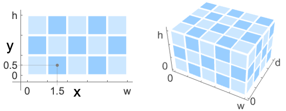
- Image and Image3D objects can also be combined with other graphics. Their pixel positions range from 0 to the dimensions of the image in the standard image coordinate system:
Examples
open all close allBasic Examples (3)
Combine the plot of a curve with the plot of a list:
Show[Plot[x ^ 2, {x, 0, 3.5}], ListPlot[{1, 4, 9}]]Combine the density plot with the contour plot:
Show[DensityPlot[Sin[x]Sin[y], {x, -3, 3}, {y, -3, 3}], ContourPlot[Sin[x]Sin[y], {x, -3, 3}, {y, -3, 3}, ContourShading -> None]]Change options for existing graphics:
Plot[Sin[x ^ 2] / x, {x, 0, 10}]Show[%, PlotRange -> {{8, 10}, {-.3, .3}}, AxesOrigin -> {8.0, 0}]Options (2)
DisplayFunction (2)
Display a graphic in PopupWindow when clicked:
Show[Graphics[{Pink, Rectangle[]}], DisplayFunction -> (PopupWindow[Button["Click here"], #]&)]Display a graphic in a new notebook:
Show[Graphics3D[{Sphere[]}], DisplayFunction -> CreateDocument]Applications (1)
Import an elevation map and take a part of it:
data = Import["http://exampledata.wolfram.com/hailey.dem.gz", "Data"];part = data[[800 ;; 1000, 800 ;; 1000]];r = ReliefPlot[part, ColorFunction -> "Rainbow", ImageSize -> 200]c = ListContourPlot[part, ContourShading -> None, Contours -> 5, ContourStyle -> {Opacity[.5], Opacity[.8]}, ImageSize -> 200]Show[r, c]Possible Issues (1)
Show uses the options from the first graphic:
Show[{PolarPlot[1 + 2 Sin[t / 2], {t, 0, π}, Ticks -> None, PlotStyle -> Red, PlotRange -> {Automatic, {0, 3}}], PolarPlot[1 + 2 Sin[t / 2], {t, π, 2 π}, Ticks -> None, PlotStyle -> Orange], PolarPlot[1 + 2 Sin[t / 2], {t, -π, 0}, Ticks -> None, PlotStyle -> Blue], PolarPlot[1 + 2 Sin[t / 2], {t, -2 π, -π}, Ticks -> None, PlotStyle -> Green]}]To see the entire graphic, use PlotRange->All:
Show[{PolarPlot[1 + 2 Sin[t / 2], {t, 0, π}, Ticks -> None, PlotStyle -> Red, PlotRange -> {Automatic, {0, 3}}], PolarPlot[1 + 2 Sin[t / 2], {t, π, 2 π}, Ticks -> None, PlotStyle -> Orange], PolarPlot[1 + 2 Sin[t / 2], {t, -π, 0}, Ticks -> None, PlotStyle -> Blue], PolarPlot[1 + 2 Sin[t / 2], {t, -2 π, -π}, Ticks -> None, PlotStyle -> Green]}, PlotRange -> All]Text
Wolfram Research (1988), Show, Wolfram Language function, https://reference.wolfram.com/language/ref/Show.html (updated 2021).
CMS
Wolfram Language. 1988. "Show." Wolfram Language & System Documentation Center. Wolfram Research. Last Modified 2021. https://reference.wolfram.com/language/ref/Show.html.
APA
Wolfram Language. (1988). Show. Wolfram Language & System Documentation Center. Retrieved from https://reference.wolfram.com/language/ref/Show.html