Wolfram Language & System Documentation Center

SystemModelLinearize

SystemModelLinearize[model]

gives a linearized StateSpaceModel for model at an equilibrium.

SystemModelLinearize[model,op]

linearizes at the operating point op.

Details and Options

SystemModelLinearize gives a linear approximation of model near an operating point.
A linear model is typically used for control design, optimization and frequency analysis.
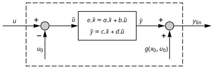
A system with equations and output equations is linearized at an operating point and that should satisfy f(0,x₀,u₀)0.

The returned linear StateSpaceModel has state , input and output , with state equations and output equation . The matrices are given by , , , and , all evaluated at , and .

SystemModelLinearize[model] is equivalent to SystemModelLinearize[model,"EquilibriumValues"].
Specifications for op use the following values for the operating point:

	"InitialValues"	initial values from model
	"EquilibriumValues"	FindSystemModelEquilibrium[model]
	sim or {sim,"StopTime"}	final values from SystemModelSimulationData sim
	{sim,"StartTime"}	initial values of sim
	{sim,time}	values at time from sim
	{{{x₁,x₁₀},…},{{u₁,u₁₀},…}}	state values x_i0 and input values u_i0

The simulation sim can be obtained using SystemModelSimulate[model,All,…].
SystemModelLinearize linearizes a system of DAEs symbolically, or first reduces it to a system of ODEs and linearizes the resulting ODEs numerically.
The following options can be given:
Method Automatic methods for linearization algorithm

ProgressReporting $ProgressReporting control display of progress
The option Method has the following possible settings:
"NumericDerivative" reduces to ODEs and then linearizes numerically

"SymbolicDerivative" linearizes symbolically from a system of DAEs
Method{"SymbolicDerivative","ReduceIndex"False} turns off index reduction.

Examples

open all close all

Basic Examples (3)

Linearize a DC-motor model around an equilibrium:

Wolfram Language code: SystemModelLinearize[[image]]

Linearize a mixing tank model around equilibrium with given state and input constraints:

Wolfram Language code: SystemModelLinearize[[image], {{{"H", 0.75}}, {{"u1", 5.23}}}]

Linearize one of the included introductory hierarchical examples:

Wolfram Language code: model = Last@SystemModelExamples["Models", "IntroductoryExamples.Hierarchical.*"]

Wolfram Language code: SystemModelLinearize[model]

Scope (19)

Model Types (5)

Linearize a textual RLC circuit model:

Wolfram Language code: SystemModelLinearize[[image]]

Linearize an RLC circuit block diagram model:

Wolfram Language code: SystemModelLinearize[[image]]

Linearize an acausal RLC circuit:

Wolfram Language code: SystemModelLinearize[[image]]

Linearize a DAE model:

Wolfram Language code: SystemModelLinearize[\!$\*GraphicsBox[«8»]$]

Linearize a DAE model symbolically:

Wolfram Language code:

SystemModelLinearize[\!\(\*GraphicsBox[«8»]\), Method -> {"SymbolicDerivative", "SymbolicParameters" -> {"R1", "R2", "L"}}]

Limiting Cases (3)

Linearize a model without inputs:

Wolfram Language code: SystemModelLinearize[[image]]

Linearize a model without states:

Wolfram Language code: SystemModelLinearize[[image]]

Linearize a model without outputs:

Wolfram Language code: SystemModelLinearize[[image]]

Linearization Values (5)

Linearize around an equilibrium:

Wolfram Language code: SystemModelLinearize[[image], "EquilibriumValues"]

Linearize around initial values:

Wolfram Language code: SystemModelLinearize[[image], "InitialValues"]

Linearize around equilibrium with given state and input constraints:

Wolfram Language code:

SystemModelLinearize[[image], {{{"H1", 2.03}, {"T1", 318.15}, {"T2", 318.15}}, {{"u1", 5}, {"u2", 5}}}, "EquilibriumValues"]

Linearize around equilibrium with state constraints:

Wolfram Language code: SystemModelLinearize[[image], {{{"H1", 5}, {"T1", 318.15}, {"T2", 318.15}}, {}}, "EquilibriumValues"]

Linearize around given partial states and inputs, using initial values for remaining values:

Wolfram Language code: SystemModelLinearize[[image], {{{"H1", 3.03}, {"T1", 318.15}, {"T2", 318.15}}, {{"u1", 5}, {"u2", 5}}}, "InitialValues"]

Operating Point (6)

Linearize around an equilibrium:

Wolfram Language code: SystemModelLinearize[[image], "EquilibriumValues"]

Linearize around initial values:

Wolfram Language code: SystemModelLinearize[[image], "InitialValues"]

Linearize around equilibrium with given state and input constraints:

Wolfram Language code:

SystemModelLinearize[[image], {{{"H1", 2.03}, {"T1", 318.15}, {"T2", 318.15}}, {{"u1", 5}, {"u2", 5}}}, "EquilibriumValues"]

Linearize around initial values from a simulation:

Wolfram Language code: sim = SystemModelSimulate[[image], All, {0, 0}]

Wolfram Language code: SystemModelLinearize[[image], {sim, "StartTime"}]

Linearize around final values from a simulation:

Wolfram Language code: sim = SystemModelSimulate[[image], All]

Wolfram Language code: SystemModelLinearize[[image], {sim, "StopTime"}]

Linearize around final values from a simulation run to steady state:

Wolfram Language code: sim = SystemModelSimulate[[image], All, Method -> {"StopAtSteadyState" -> True}]

Wolfram Language code: SystemModelLinearize[[image], {sim, "StopTime"}]

Generalizations & Extensions (1)

Hide labels in the resulting StateSpaceModel:

Wolfram Language code: SystemModelLinearize[[image], SystemsModelLabels -> None]

Options (5)

Method (4)

The "SymbolicDerivative" method uses a fully specified operating point from a simulation:

Wolfram Language code: sim = SystemModelSimulate[[image], All, {0, 0}]

Wolfram Language code: SystemModelLinearize[[image], sim, Method -> "SymbolicDerivative"]

The "NumericDerivative" method uses an operating point specified by state and input values:

Wolfram Language code: SystemModelLinearize[[image], {{{"capacitor.v", 0.}, {"inductor.i", 0.}}, {{"v", 0.}}}, Method -> "NumericDerivative"]

Linearizing symbolically allows keeping some parameters symbolic:

Wolfram Language code: SystemModelLinearize[[image], Method -> {"SymbolicDerivative", "SymbolicParameters" -> {"R", "L", "C"}}]

Use "ReduceIndex" to turn off index reduction when linearizing symbolically:

Wolfram Language code: sim = SystemModelSimulate[[image], All, {0, 0}];

Turning off index reduction results in a descriptor StateSpaceModel:

Wolfram Language code: SystemModelLinearize[[image], sim, Method -> {"SymbolicDerivative", "ReduceIndex" -> False}]

ProgressReporting (1)

Control progress reporting with ProgressReporting:

Wolfram Language code: SystemModelLinearize[[image], ProgressReporting -> False]

Applications (10)

Analyzing Linearized System (5)

Compare responses from a model and its linearization at an equilibrium point:

Wolfram Language code: model = [image];

Wolfram Language code: {Subscript[x, 0], Subscript[u, 0], Subscript[y, 0]} = FindSystemModelEquilibrium[model];

Linearize around the equilibrium point:

Wolfram Language code: ss = SystemModelLinearize[model, "EquilibriumValues"];

Compare the stationary output response with a nonlinear model:

Wolfram Language code: {linY1, linY2} = OutputResponse[ss, {UnitStep[t], UnitStep[t]}, {t, 0, 300}];

Wolfram Language code:

nonLin = SystemModelSimulate[model, {0, 300}, <|"InitialValues" -> Rule@@@Subscript[x, 0], "Inputs" -> {"u1" -> Function[t, Subscript[u, 0][[1, 2]] + UnitStep[t]], "u2" -> Function[t, Subscript[u, 0][[2, 2]] + UnitStep[t]]}|>];

Compare the y1 output:

Wolfram Language code: Show[SystemModelPlot[nonLin, {"y1"}], Plot[Tooltip[Subscript[y, 0][[1, 2]] + linY1, "linear y1"], {t, 0, 300}]]

Test the stability of a linearized system from eigenvalues of the system matrix:

Wolfram Language code: ss = SystemModelLinearize[[image], "InitialValues"]

Since there is an eigenvalue with a positive real part, the system is unstable:

Wolfram Language code: {a, b, c, d} = Normal[ss];

Wolfram Language code: Re@Eigenvalues[a]

Plotting the output response also indicates an unstable system:

Wolfram Language code: Plot[Evaluate[OutputResponse[ss, UnitStep[t], {t, 1}]], {t, 0, 1}]

Test the stability of a linearized system from poles of the transfer function:

Wolfram Language code: tf = TransferFunctionModel@SystemModelLinearize[[image]];

Since there is a pole with a positive real part, the system is unstable:

Wolfram Language code: TransferFunctionPoles[tf]

Do a frequency analysis using a linear model:

Wolfram Language code: model = \!$\*GraphicsBox[«8»]$;

By plotting for the linearized transfer function :

Wolfram Language code: ss = SystemModelLinearize[model];

Wolfram Language code: BodePlot[ss, {0.5, 3}, PlotLayout -> "Magnitude"]

Verify the result using Fourier on simulated data:

Wolfram Language code: nonLin = SystemModelSimulate[model, {0, 200}, <|"Inputs" -> {"u" -> Function[t, UnitStep[t] - UnitStep[t - 2]]}|>];

Compute from :

Wolfram Language code:

odata = Abs@Fourier@Table[nonLin[{"inertia3.w"}, t][[1]], {t, 0, 200, 0.25}];
idata = Abs@Fourier@Table[UnitStep[t] - UnitStep[t - 2], {t, 0, 200, 0.25}];

Wolfram Language code:

ListLogLinearPlot[odata[[1 ;; 200]] / idata[[1 ;; 200]], Joined -> True, DataRange -> {0, 2Pi}, PlotRange -> {{0.5, 3}, {0, 50}}]

Alternatively, the imaginary parts of the eigenvalues give the resonance peaks:

Wolfram Language code: {a, b, c, d} = Normal[ss];

Wolfram Language code: Im[Eigenvalues[a]]

Linearization takes place at time 0:

Wolfram Language code: model = [image];

Linearize with the switch connecting at time 0:

Wolfram Language code: model2 = SystemModel[model, {"t" -> 0}];

Wolfram Language code: rlc = SystemModelLinearize[model2]

If the switch is not connected at time 0, the result is different:

Wolfram Language code: model3 = SystemModel[model2, {"t" -> 1}];

Wolfram Language code: rl = SystemModelLinearize[model3]

Controller Design for Linearized System (5)

Design a PID controller using a linearized model:

Wolfram Language code: tf = TransferFunctionModel@SystemModelLinearize[[image]];

Define a PID controller and closed-loop transfer function:

Wolfram Language code: pidTf = TransferFunctionModel[kp (1 + 1 / (τi ) + τd ), ];

Wolfram Language code: cltf = SystemsModelFeedbackConnect[SystemsModelSeriesConnect[pidTf, tf]];

Select PID parameters for appropriate step response:

Wolfram Language code:

Manipulate[
	Plot[OutputResponse[cltf /. {kp -> gain, τi -> iTime, τd -> dTime}, UnitStep[t], {t, 20}]//Evaluate, {t, 0, 20}, PlotStyle -> Thick, GridLines -> Automatic, Frame -> True, PlotRange -> {0, 1.2}], 
	{{gain, 1, "SubscriptBox[k, p]"}, 0.01, 10}, {{dTime, 0.01, "SubscriptBox[τ, d]"}, 0.01, 10}, {{iTime, 1.9, "SubscriptBox[τ, i]"}, 0.01, 10}, SaveDefinitions -> True]

Design a lead-based controller for a DC motor based on its linearization:

Wolfram Language code: tf = TransferFunctionModel@SystemModelLinearize[[image]];

Define a PI-lead controller transfer function:

Wolfram Language code: piLeadTf = TransferFunctionModel[kp (1 + 1 / τi (τd  + 1) / (α τd  + 1)), ];

Open-loop transfer function:

Wolfram Language code: optf = SystemsModelSeriesConnect[piLeadTf, tf];

Select controller parameters:

Wolfram Language code:

Manipulate[BodePlot[newOptf = optf /. {kp -> Kp, τi -> Τi, τd -> Τd, α -> Α}, StabilityMargins -> True, PlotLayout -> "List"], 
	{{Kp, 4.5, "SubscriptBox[k, p]"}, 0.01, 10}, {{Τi, 2, "τi"}, 0.01, 10}, {{Τd, 0.01, "τd"}, 0.01, 10}, {{Α, 0.07, "α"}, 0.01, 0.9}, SaveDefinitions -> True]

Use selected parameters and close the loop with the PI-lead controller:

Wolfram Language code: cltf = SystemsModelFeedbackConnect[SystemsModelSeriesConnect[newOptf, tf]];

Wolfram Language code:

Plot[OutputResponse[cltf, UnitStep[t], {t, 20}]//Evaluate, {t, 0, 20}, PlotStyle -> Thick, GridLines -> Automatic, Frame -> True, PlotRange -> All]

Design a controller using pole placement:

Wolfram Language code: ss = SystemModelLinearize[[image]];

Place the closed-loop poles:

Wolfram Language code: k = StateFeedbackGains[ss, {-0.251, -0.222, -0.222}]

Compute the closed-loop state-space model:

Wolfram Language code: clss = SystemsModelStateFeedbackConnect[ss, k];

Show the step response:

Wolfram Language code: Plot[OutputResponse[clss, {UnitStep[t], UnitStep[t]}, {t, 100}]//Evaluate, {t, 0, 100}, PlotRange -> All]

Design an LQ controller:

Wolfram Language code: ss = SystemModelLinearize[[image]];

Define state and input weight matrices:

Wolfram Language code: {q1, q2} = {DiagonalMatrix[{1, 6 10^-4, 6 10^-4}], DiagonalMatrix[{0.0002, 0.0002}]};

Define LQ controller gain:

Wolfram Language code: k = LQRegulatorGains[ss, {q1, q2}]

Closed-loop state-space model:

Wolfram Language code: clss = SystemsModelStateFeedbackConnect[ss, k];

Closed-loop step response:

Wolfram Language code: Plot[OutputResponse[clss, {UnitStep[t], UnitStep[t]}, {t, 100}]//Evaluate, {t, 0, 100}, PlotRange -> All]

Design a state estimator:

Wolfram Language code: model = [image];

Wolfram Language code: ss = SystemModelLinearize[model];

Compute estimator gains and the estimator state-space model:

Wolfram Language code: l = EstimatorGains[ss, {-0.6020, -0.5856, -0.5697}]

Wolfram Language code: {a, b, c, d} = Normal[ss];

Wolfram Language code: ssobsv = StateSpaceModel[{a - l.c, ArrayFlatten[{{b - l.d, l}}], IdentityMatrix[3]}];

The state and output response to a unit step on the inputs:

Wolfram Language code: sresp = StateResponse[ss, {UnitStep[t], UnitStep[t]}, {t, 200}];

Wolfram Language code: y = OutputResponse[ss, {UnitStep[t], UnitStep[t]}, {t, 200}];

Observer state response:

Wolfram Language code: oresp = OutputResponse[ssobsv, {UnitStep[t], UnitStep[t], y[[1]], y[[2]]}, {t, 200}];

Compare each state and its estimate:

Wolfram Language code: states = model["StateVariables"];

Wolfram Language code: Table[Plot[{sresp[[i]], oresp[[i]]}, {t, 0, 200}, PlotLabel -> states[[i]]], {i, 3}]

Properties & Relations (7)

Linearize around initial values using properties from SystemModel:

Wolfram Language code: model = [image];

Wolfram Language code: ival = model["GroupedInitialValues"]

Compare results:

Wolfram Language code: SystemModelLinearize[model, ival, "InitialValues"] == SystemModelLinearize[model, "InitialValues"]

Linearize around equilibrium using FindSystemModelEquilibrium:

Wolfram Language code: model = [image];

Wolfram Language code: eqval = FindSystemModelEquilibrium[model];

Compare results:

Wolfram Language code: SystemModelLinearize[model, eqval] == SystemModelLinearize[model, "EquilibriumValues"]

Compare responses from a model and its linearization at an equilibrium point:

Wolfram Language code: model = [image];

Wolfram Language code:

{Subscript[x, 0], Subscript[u, 0], Subscript[y, 0]} = FindSystemModelEquilibrium[model, {"H" == 0.85, "Tu" == 38, "Tx" == 38}]

Linearize around the equilibrium point:

Wolfram Language code: ss = SystemModelLinearize[model, {{{"H", 0.85}, {"Tu", 38}, {"Tx", 38}}, {}}, "EquilibriumValues"]

Compare the stationary output response with a nonlinear model:

Wolfram Language code: {linY1, linY2} = OutputResponse[ss, {UnitStep[t], UnitStep[t]}, {t, 0, 300}];

Wolfram Language code:

nonLin = SystemModelSimulate[model, {0, 300}, <|"InitialValues" -> Rule@@@Subscript[x, 0], "Inputs" -> {"u1" -> Function[t, Subscript[u, 0][[1, 2]] + UnitStep[t]], "u2" -> Function[t, Subscript[u, 0][[2, 2]] + UnitStep[t]]}|>];

Compare the first output:

Wolfram Language code: Show[SystemModelPlot[nonLin, {"y1"}], Plot[Evaluate@Tooltip[Subscript[y, 0][[1, 2]] + linY1, "linear y1"], {t, 0, 300}]]

Use TransferFunctionModel to convert to a transfer function representation:

Wolfram Language code: SystemModelLinearize[[image]]

Wolfram Language code: TransferFunctionModel[%]

Use ToDiscreteTimeModel to discretize a linearized model:

Wolfram Language code: SystemModelLinearize[[image]]

Discretize using sample time :

Wolfram Language code: ToDiscreteTimeModel[%, 0.10, z]

The linearized state-space model is not unique:

Wolfram Language code: linearize1 = [image];

Wolfram Language code: linearize1["ModelicaDisplay"]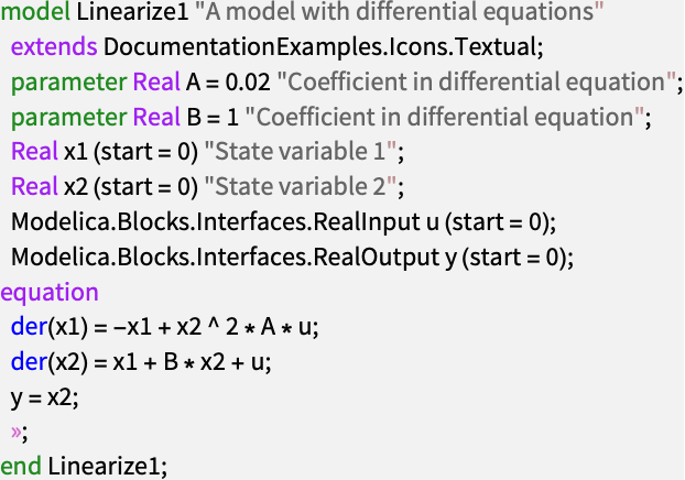

Wolfram Language code: ss1 = SystemModelLinearize[linearize1]

Change the order in which the variables x1 and x2 are declared:

Wolfram Language code: linearize2 = [image];

Wolfram Language code: linearize2["ModelicaDisplay"]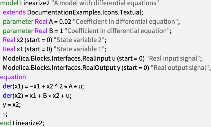

Wolfram Language code: ss2 = SystemModelLinearize[linearize2]

The models are equivalent and have identical transfer functions:

Wolfram Language code: TransferFunctionModel[ss1] == TransferFunctionModel[ss2]

StateSpaceModel can linearize systems of ordinary differential equations:

Wolfram Language code: ClearAll[t, x, θ, i, vin, g, r, lin, mc, mp, l, k, dc, dp, a];

Wolfram Language code:

eqs = {(mc + mp)x''[t] - mp l Cos[θ[t]] θ''[t] + mp l Sin[θ[t]] θ'[t]^2 == k i[t] - dc x'[t], θ''[t]mp (4l^2  / 3 + a^2 / 4) - mp l x''[t] Cos[θ[t]] == mp g l Sin[θ[t]] - dp θ'[t], 0 == vin[t] - r i[t] - lin i'[t] - k x'[t]};

Wolfram Language code: opssm = Sequence[{{i[t], 0}, {θ[t], 0}, {θ'[t], 0}, {x[t], 0}, {x'[t], 0}}, {{vin[t], 0}}];

Wolfram Language code: outputs = {θ[t], x[t]};

Wolfram Language code: ssm = StateSpaceModel[eqs, opssm, outputs, t]//Simplify

Use approximate numeric parameter values:

Wolfram Language code:

parVals = {g -> 9.80665, r -> 13, lin -> 1, mc -> 445 * 0.1^3, mp -> 7700 * π * 0.005^2 * 0.61, l -> 0.61 / 2, a -> 0.005, k -> 3.7 * 157.48 * 1.6, dc -> 2, dp -> 0.01};

Wolfram Language code: ssm /. parVals

Use SystemModelLinearize to linearize a SystemModel of the same system:

Wolfram Language code: model = SystemModel[[image], <|"ParameterValues" -> {"electricalMotor.J" -> 0}|>];

Wolfram Language code: op = FindSystemModelEquilibrium[model]

Wolfram Language code: SystemModelLinearize[model, op]

Create a NonlinearStateSpaceModel from the equations and compare with the SystemModel:

Wolfram Language code: nssm = NonlinearStateSpaceModel[eqs, opssm, outputs, t]//Simplify

Wolfram Language code:

plotComparison[nssmVar_, smVar_] := Show[SystemModelPlot[nssm, {nssmVar}, 20, <|"ParameterValues" -> parVals, "Inputs" -> {vin -> UnitBox}|>, PlotLabel -> nssmVar, ...], SystemModelPlot[model, {smVar}, 20, <|"Inputs" -> {"V" -> UnitBox}|>, TargetUnits -> "Unit", ...]];

Wolfram Language code: plotComparison[θ, "pendulum.pendulumDamper.phi_rel"]

Wolfram Language code: plotComparison[x, "pendulum.sliderConstraint.s"]

Possible Issues (1)

Some models cannot be linearized symbolically:

Wolfram Language code: SystemModelLinearize["DocumentationExamples.Modeling.ElectricCircuit.CircuitWithEvent", Method -> "SymbolicDerivative"]

Wolfram Language code: SystemModelLinearize["DocumentationExamples.Basic.StateOut", Method -> "SymbolicDerivative"]

Wolfram Language code: SystemModelLinearize["DocumentationExamples.Basic.InOutNoState", Method -> "SymbolicDerivative"]

Use "NumericDerivative" to linearize numerically:

Wolfram Language code: SystemModelLinearize["DocumentationExamples.Modeling.ElectricCircuit.CircuitWithEvent", Method -> "NumericDerivative"]

Top

More Learning

Tech Support

Wolfram Solutions

Wolfram Solutions For Education

Get Started

Grow Your Skills

Work with Us

Educational Programs for Adults

Educational Programs for Youth

Read

SystemModelLinearize

Details and Options

Examples

Basic Examples (3)

Scope (19)

Model Types (5)

Limiting Cases (3)

Linearization Values (5)

Operating Point (6)

Generalizations & Extensions (1)

Options (5)

Method (4)

ProgressReporting (1)

Applications (10)

Analyzing Linearized System (5)

Controller Design for Linearized System (5)

Properties & Relations (7)

Possible Issues (1)

Text

CMS

APA

BibTeX

BibLaTeX

	Method	Automatic	methods for linearization algorithm
	ProgressReporting	$ProgressReporting	control display of progress

SystemModelLinearize

Details and Options

Examples

Basic Examples (3)

Scope (19)

Model Types (5)

Limiting Cases (3)

Linearization Values (5)

Operating Point (6)

Generalizations & Extensions (1)

Options (5)

Method (4)

ProgressReporting (1)

Applications (10)

Analyzing Linearized System (5)

Controller Design for Linearized System (5)

Properties & Relations (7)

Possible Issues (1)

See Also

Related Guides

Related Links

History

Text

CMS

APA

BibTeX

BibLaTeX