TransferFunctionModel is typically used for signal filters and control design.
A continuous-time system modeled by where is the Laplace transform of the output, is the Laplace transform of the input and is the transfer matrix can be specified as TransferFunctionModel[g[s],s].

A discrete-time system modeled by where is the Z transform of the output, is the Z transform of the input and is the transfer matrix can be specified as TransferFunctionModel[g[z],z,SamplingPeriodτ].

Time delays can be included in any transfer-function model, by using SystemsModelDelay.
In TransferFunctionModel[sys], the following systems can be converted:
AffineStateSpaceModel approximate Taylor conversion

NonlinearStateSpaceModel approximate Taylor conversion

StateSpaceModel exact conversion
TransferFunctionModel[…]["prop"] gives the value of the property "prop".
TransferFunctionModel[…]["Properties"] gives the list of available properties.
The following options can be given:

Appearance	Automatic	model appearance
Method	Automatic	the method to obtain the transfer function of a state-space model
SamplingPeriod	Automatic	the sampling period of the system
SystemsModelLabels	Automatic	labels for the input and output variables
ExternalTypeSignature	Automatic	variable types for embedded code

The option Appearance can take values Automatic, "Detailed", "Structured", "Elided", and "Iconized".
Settings for the Method option include "DeterminantExpansion", "ResolventIdentities", "Inverse", and "Generic". With a setting Method->Automatic, the transfer-function model is computed using determinant expansion.

Examples

open all close all

Basic Examples (5)

A single-input, single-output system:

Wolfram Language code: TransferFunctionModel[{{(1/s)}}, s]

A system with two inputs and one output:

Wolfram Language code: TransferFunctionModel[{{(2/1 + s^2), (s/s - 1)}}, s]

Obtain the transfer-function representation of a state-space model:

Wolfram Language code:

TransferFunctionModel[StateSpaceModel[{{{a}}, {{b}}, {{c}}, {{0}}}, 
 SamplingPeriod -> None, SystemsModelLabels -> None]]

A discrete-time transfer function with a sampling period of 1:

Wolfram Language code: TransferFunctionModel[(1/(z - 1)(z - 0.605)), z, SamplingPeriod -> 1]

Evaluate a transfer function over a range of frequencies:

Wolfram Language code:

tfm = TransferFunctionModel[(s + 0.25/s^2 + s + 1), s];
tfm[I Range[0.01, 5, 0.5]]

Plot the magnitudes:

Wolfram Language code: Plot[Abs[tfm[I f]], {f, 0, 5}]

Scope (19)

A first-order continuous-time system:

Wolfram Language code: TransferFunctionModel[(1/T s + 1), s]

A second-order system:

Wolfram Language code: TransferFunctionModel[(Subsuperscript[ω, n, 2]/s^2 + 2ζ Subscript[ω, n] s + Subsuperscript[ω, n, 2]), s]

A fifth-order system:

Wolfram Language code:

TransferFunctionModel[k (Subsuperscript[∑, i = 0, 2]Subscript[b, i]s^i/Subsuperscript[∑, i = 0, 5]Subscript[a, i]s^i), s]

A system with three zeros and six poles:

Wolfram Language code:

TransferFunctionModel[k (Subsuperscript[∏, i = 1, 3](s + Subscript[z, i])/(Subsuperscript[∏, i = 1, 2](s + Subscript[p, i]))Subsuperscript[∏, i = 1, 2](s^2 + 2 Subscript[ξ, i]Subscript[ω, i]s + Subsuperscript[ω, i, 2])), s]

A first-order discrete-time system:

Wolfram Language code: TransferFunctionModel[(1/z - 1), z, SamplingPeriod -> τ]

A two-input, one-output system:

Wolfram Language code: TransferFunctionModel[{{(1/s), (1/s + 1)}}, s]

Wolfram Language code: SystemsModelDimensions[%]

A one-input, two-output system:

Wolfram Language code: TransferFunctionModel[{{(1/s)}, {(1/s + 1)}}, s]

Wolfram Language code: SystemsModelDimensions[%]

A two-input, two-output system:

Wolfram Language code: TransferFunctionModel[{{(1/s), (1/s + 1)}, {(1/s + 2), (1/s + 3)}}, s]

Wolfram Language code: SystemsModelDimensions[%]

Specify a transfer function using its numerator and denominator:

Wolfram Language code: TransferFunctionModel[{{{1}}, {{s + 1}}}, s]

A MIMO transfer function specified in terms of its numerators and denominators:

Wolfram Language code: TransferFunctionModel[{{{1, s}, {s + 2, s + 4}}, {{s - 5, s + 3}, {s - 1, s + 4}}}, s]

A denominator polynomial that is the least common multiple:

Wolfram Language code: TransferFunctionModel[{{{3(s + 1), s + 6}, {s + 3, s + 2}}, (s + 1)(s + 2)}, s]

Specify the transfer function, using its algebraic poles, zeros, and gains:

Wolfram Language code: TransferFunctionModel[{{{{z}}}, {{{p}}}, {{g}}}, s]

A multivariable system:

Wolfram Language code:

TransferFunctionModel[{(|       |       |
| ----- | ----- |
| {z11} | {z12} |
| {z21} | {z22} |), (|       |       |
| ----- | ----- |
| {p11} | {p12} |
| {p21} | {p22} |), (|     |     |
| --- | --- |
| g11 | g12 |
| g21 | g22 |)}, s]

A constant gain of 10:

Wolfram Language code: TransferFunctionModel[10]

A discrete-time gain:

Wolfram Language code: TransferFunctionModel[10, SamplingPeriod -> 1]

A symbolic gain:

Wolfram Language code: TransferFunctionModel[g]

Wolfram Language code: % /. g -> 5

The transfer-function representation of a state-space model:

Wolfram Language code:

TransferFunctionModel[StateSpaceModel[{{{-3, 0}, {0, -2}}, {{1}, {2}}, {{1, 0}}, {{0}}}, SamplingPeriod -> None, 
 SystemsModelLabels -> None], s]

Taylor linearize an AffineStateSpaceModel and obtain its transfer function representation:

Wolfram Language code:

TransferFunctionModel[AffineStateSpaceModel[{{Subscript[x, 1] + Subscript[x, 2]^2, 
   (-Subscript[x, 1])*Subscript[x, 2]}, 
  {{1}, {Subscript[x, 1]}}, {Subscript[x, 1]}, {{0}}}, 
 {Subscript[x, 1], Subscript[x, 2]}, {u}, {Automatic}, 
 Automatic, SamplingPeriod -> None], s]

The linearization of an AffineStateSpaceModel with nonzero equilibrium values:

Wolfram Language code:

TransferFunctionModel[AffineStateSpaceModel[{{Subscript[x, 1] + 2*Subscript[x, 2] + 
    Subscript[x, 2]^2, 1 - Subscript[x, 1] + 
    Subscript[x, 2] - Subscript[x, 1]*Subscript[x, 2]}, 
  {{1}, {Subscript[x, 1]}}, {-1 + Subscript[x, 1]}, {{0}}}, 
 {{Subscript[x, 1], 1}, {Subscript[x, 2], -1}}, {u}, 
 {Automatic}, Automatic, SamplingPeriod -> None], s]

Taylor linearize a NonlinearStateSpaceModel:

Wolfram Language code:

TransferFunctionModel[NonlinearStateSpaceModel[{{-1 + u*x}, {-1 + x}}, 
 {{x, 1}}, {{u, 1}}, {Automatic}, Automatic, SamplingPeriod -> None], s]

The list of available properties:

Wolfram Language code: TransferFunctionModel[{{{3 + s}}, 10 + 7*s + s^2}, s]["Properties"]

Generalizations & Extensions (2)

SISO systems can also be specified as a single-element list:

Wolfram Language code: TransferFunctionModel[{(1/s)}, s]

Or just as a rational function:

Wolfram Language code: TransferFunctionModel[(1/s), s]

A single-output system can be given as a list:

Wolfram Language code: TransferFunctionModel[{(1/2 s + 1), (3/4 s + 1)}, s]

Options (5)

SamplingPeriod (3)

Specify a continuous-time system:

Wolfram Language code: TransferFunctionModel[(1/s^2 + a s + b), s]

Wolfram Language code: TransferFunctionModel[(1/s^2 + a s + b), s, SamplingPeriod -> None]

A discrete-time system with sampling period 1:

Wolfram Language code: TransferFunctionModel[(z/z - 1), z, SamplingPeriod -> 1]

A system with a symbolic sampling period:

Wolfram Language code: TransferFunctionModel[(1/s^2 + a s + b), s, SamplingPeriod -> T]

Set the sampling period to a numeric value:

Wolfram Language code: % /. T -> 2

SystemsModelLabels (1)

Label the input and output variables of a transfer function model:

Wolfram Language code:

TransferFunctionModel[(⁠|             |           |             |
| ----------- | --------- | ----------- |
| (s/2 + s^2) | (1/s)     | (1/2 + s^2) |
| (1/s)       | (1 + s/s) | (1/2 + s^2) |⁠), s, SystemsModelLabels -> {{"SubscriptBox[u, 1]", "SubscriptBox[u, 2]", "SubscriptBox[u, 3]"}, {"SubscriptBox[y, 1]", "SubscriptBox[y, 2]"}}]

By default, the appearance is selected to fit the display in the notebook:

Wolfram Language code:

TransferFunctionModel[{{(18/(s + 1)(s + 3)(s + 6)), (10/(s + 5)(s + 2)), (3/s^3 + s^2 + s + 3), (2/s(s + 1)(s + 2))}, {(100/s^2 + 3s + 100), (3/s(s + 1)(s + 3)(s + 6)), (3/s^3 + s^2 + s + 3), (4/(s + 1)(s + 2)(s + 5)(s + 3))}, {(20/(s + 5)(s + 4)), (10/s^2 + 10), (5/s^2 + s + 5), (10/s^4 + 5 s^2 + 10)}}, s]

Wolfram Language code: TransferFunctionModel[(1/s + 1), s]

Applications (18)

A proportional-integral (PI) controller:

Wolfram Language code: TransferFunctionModel[Subscript[k, p] + (Subscript[k, i]/ s), s]

A proportional-derivative (PD) controller:

Wolfram Language code: TransferFunctionModel[Subscript[k, p] + Subscript[k, d] s, s]

A function to construct a proportional-integral-derivative (PID) controller:

Wolfram Language code: pid[kp_, ki_, kd_] := TransferFunctionModel[kp + (ki/ s) + kd s, s]

A PID with specific gain values:

Wolfram Language code: pid[1, 2.5, 0.5]

A function to construct a discrete-time PID controller:

Wolfram Language code: dpid[kp_, ki_, kd_, τ_] := TransferFunctionModel[kp + ki(τ z/z - 1) + kd (z - 1/τ z), z, SamplingPeriod -> τ]

Wolfram Language code: dpid[260, 130, 5, 0.1]

A function for a continuous-time lead compensator:

Wolfram Language code: lead[k_, T_ /; T > 0, α_ /; 0 < α < 1] := TransferFunctionModel[k(s + (1/T)/ s + (1/α T)), s]

A lead compensator for specific values of gain and pole-zero locations:

Wolfram Language code: lead[200, 0.02, 0.5]

A function for a continuous-time lag compensator:

Wolfram Language code: lag[k_, T_ /; T > 0, α_ /; α > 1] := TransferFunctionModel[k(s + (1/T)/ s + (1/α T)), s]

A specific lag compensator:

Wolfram Language code: lag[1000, 0.08, 2]

A digital lag compensator defined in terms of its zero and pole locations:

Wolfram Language code:

dlag[zero_, pole_, τ_] /; zero < pole < 1 := TransferFunctionModel[((1 - pole)(z - zero)/ (1 - zero)(z - pole)), z, SamplingPeriod -> τ];

Wolfram Language code: dlag[0.2, 0.5, 0.01]

A general formula for analog lowpass Butterworth filters:

Wolfram Language code:

butterworth[ω_, n_ ? OddQ] := TransferFunctionModel[(ω/s + ω)Underoverscript[∏, i = 1, (n - 1) / 2](ω^2/s^2 + 2Cos[(π i/n)]ω s + ω^2), s]
butterworth[ω_, n_] := TransferFunctionModel[Underoverscript[∏, i = 1, n / 2](ω^2/s^2 + 2Cos[(π (i - 1 / 2)/n)]ω s + ω^2), s]

Filters of specific orders:

Wolfram Language code: butterworth[Subscript[ω, N], 3]

Wolfram Language code: butterworth[Subscript[ω, N], 4]//N

A third-order Bessel filter:

Wolfram Language code: TransferFunctionModel[(15/ s^3 + 6s^2 + 15 s + 15), s]

The general second-order transfer function:

Wolfram Language code: order2[ζ_, ω_] := TransferFunctionModel[ (ω^2/s^2 + 2ζ ω s + ω^2), s];

Variations in damping ratio lead to qualitatively different responses:

Wolfram Language code:

Table[{Last[damping], sys = order2[First[damping], 6], Plot[OutputResponse[sys, UnitStep[t], t]//Evaluate, {t, 0, 8}, PlotRange -> All]}, {damping, {{0, "Undamped"}, {0.7, "Underdamped"}, {1, "Critically damped"}, {5, "Overdamped"}}}]//TableForm

A linearized inverted pendulum model:

Wolfram Language code:

invpend[M_, m_, l_, g_] := TransferFunctionModel[{{{-s^2}, { l s^2 - g}, {-s^3}, {l s^3 - g s}}, M l s^4 - g(M + m)s^2}, s, SystemsModelLabels -> {"u", {"θ", "x", "θ'", "x'"}}]

Wolfram Language code: invpend[5, 3.75, 1.5, 9.8]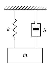

A spring-mass-damper system:

Wolfram Language code: smd[k_, m_, b_] := TransferFunctionModel[ (1/m s^2 + b s + k), s];

Wolfram Language code: smd[0.1, 0.5, 0.2]

Transfer function between the input voltage and the shaft angular position of a DC motor:

Wolfram Language code: dcmotor[Kt_, Kf_, J_, B_, L_, R_] := TransferFunctionModel[ (Kt/(J s^2 + B s)(L s + R) + Kt Kf s), s];

Wolfram Language code: dcmotor[0.02, 0.02, 0.015, 0.1, 0.5, 1.3]

The aileron-to-roll-rate transfer function of an aircraft:

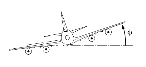
Wolfram Language code: TransferFunctionModel[(-5.9(s - 0.05)(s^2 + 0.46s + 1.1978)/(s + 0.067)(s + 0.7)(s^2 + 0.8054s + 4.21031)), s]

A temperature-controlled chemical reactor:

Wolfram Language code: TransferFunctionModel[(Subscript[k, p]/1 + Subscript[τ, p] s), s]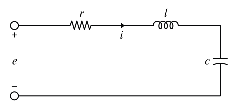

An RLC circuit:

Wolfram Language code: rlc[r_, l_, c_] := TransferFunctionModel[(r/r + s l + (1/s c)), s];

Wolfram Language code: rlc[100, 10^-4, 10^-6]

A MIMO transfer function describing an aircraft's longitudinal dynamics:

Wolfram Language code:

TransferFunctionModel[{{(-0.0005(s - 70)(s + 0.5)/(s^2 + 0.0065s + 0.006)(s^2 + s + 1.4))}, {(-0.02(s + 80)(s^2 + 0.0065s + 0.006)/(s^2 + 0.005s + 0.006)(s^2 + s + 1.4))}, {(-1.4(s + 0.02)(s + 0.4)/(s^2 + 0.005s + 0.006)(s^2 + s + 1.4))}}, s]

A ball mill grinding system with delay due to material transport:

Wolfram Language code:

TransferFunctionModel[{{{-0.425 / E ^ (1.52 * s), 0.1052 * (1 + 47.1 * s)}, 
    {2.977, 1.063 / E ^ (2.26 * s)}}, {{1 + 11.7 * s, 1 + 11.5 * s}, {1 + 5.5 * s, 1 + 2.5 * s}}}, s, 
  SystemsModelLabels -> {{"FreshFeed", "SumpWater"}, {"Product", "Throughput"}}]

Properties & Relations (6)

TransferFunctionModel behaves as a pure function of one argument:

Wolfram Language code: lsys = TransferFunctionModel[{{(2/1 + s^2), (s/s - 1)}}, s]

Wolfram Language code: lsys[x]

The value of the transfer-function matrix at a specific frequency:

Wolfram Language code: lsys[10. I]

The values at several frequencies:

Wolfram Language code: lsys[Range[3, 7]I]

Use TransferFunctionFactor to obtain the factored form:

Wolfram Language code: TransferFunctionFactor[TransferFunctionModel[(1/s) + (1/s - 1), s]]

Obtain the expanded form:

Wolfram Language code: TransferFunctionExpand[TransferFunctionModel[(1/s) + (1/s - 1), s]]

Use TransferFunctionCancel to cancel any common poles and zeros:

Wolfram Language code: TransferFunctionModel[{{{s + 10}}, (s + 10)}, s]

Wolfram Language code: TransferFunctionCancel[%]

Find the element zeros and poles of a transfer-function matrix:

Wolfram Language code:

tfm = TransferFunctionModel[{{(s/1 + s^2), (s + 3/s - 1), (1/s + 1)}, {(s - 3/s + 2), (s + 1/s + 2), (s + 4/1 + s^2)}}, s];

Wolfram Language code: TransferFunctionPoles[tfm]

Wolfram Language code: TransferFunctionZeros[tfm]

Obtain a state-space form of a transfer-function model:

Wolfram Language code: StateSpaceModel[ TransferFunctionModel[{{(10(s - 2)/(s^2 + 2 s + 1.25) (s^2 + 6 s + 25))}}, s]]

Possible Issues (3)

In TransferFunctionModel[m,var], pole-zero pairs may cancel before being processed:

Wolfram Language code: ((s + 2)(s + 3)/(s + 2)(s + 4))

Wolfram Language code: TransferFunctionModel[((s + 2)(s + 3)/(s + 2)(s + 4)), s]

Use Unevaluated to prevent cancellations:

Wolfram Language code: TransferFunctionModel[Unevaluated[((s + 2)(s + 3)/(s + 2)(s + 4))], s]

Or use TransferFunctionModel[{num,den},var]:

Wolfram Language code: TransferFunctionModel[{{{(s + 2)(s + 3)}}, (s + 2)(s + 4)}, s]

Or TransferFunctionModel[{z,p,g},var]:

Wolfram Language code: TransferFunctionModel[{{{{-3, -2}}}, {-4, -2}, {{1}}}, s]

TransferFunctionModel[m,var] might result in a system with higher order:

Wolfram Language code:

m = (1/(s + 1)) - (1/(s + 1)^2);
TransferFunctionModel[m, s]

Simplify the system:

Wolfram Language code: TransferFunctionModel[%, s]//Simplify

Or simplify m before passing it to TransferFunctionModel:

Wolfram Language code: Together[m]

Wolfram Language code: TransferFunctionModel[%, s]

If the complex variable var is not specified, it is assumed to be s for continuous-time systems:

Wolfram Language code: TransferFunctionModel[(s/10s + 1)]

Wolfram Language code: %[var]

Specify the transfer function using s:

Wolfram Language code: TransferFunctionModel[(/10 + 1)][var]

For discrete-time systems, use z:

Wolfram Language code: TransferFunctionModel[(1/ + 0.4), SamplingPeriod -> τ][var]

Top

More Learning

Tech Support

Wolfram Solutions

Wolfram Solutions For Education

Get Started

Grow Your Skills

Work with Us

Educational Programs for Adults

Educational Programs for Youth

Read

TransferFunctionModel

Details and Options

Examples

Basic Examples (5)

Scope (19)

Generalizations & Extensions (2)

Options (5)

SamplingPeriod (3)

SystemsModelLabels (1)

Applications (18)

Properties & Relations (6)

Possible Issues (3)

Text

CMS

APA

BibTeX

BibLaTeX

	AffineStateSpaceModel	approximate Taylor conversion
	NonlinearStateSpaceModel	approximate Taylor conversion
	StateSpaceModel	exact conversion

TransferFunctionModel

Details and Options

Examples

Basic Examples (5)

Scope (19)

Generalizations & Extensions (2)

Options (5)

SamplingPeriod (3)

SystemsModelLabels (1)

Applications (18)

Properties & Relations (6)

Possible Issues (3)

See Also

Related Guides

History

Text

CMS

APA

BibTeX

BibLaTeX