Slope Stability
| Introduction | Shear Strength Reduction |
| Geometry and Load Scheme | Slope Angle |
| Soil Behavior | 3D Visualization |
| Slope Failure Zones | References |
Introduction
A ground surface that is inclined at an angle to the horizontal is called a slope. Slopes are formed by inclining soil masses and can occur naturally or can be manmade. Slopes are commonly required in the construction of highways, railway embankments, earth dams, levees and canals.
When the ground surface is inclined, the gravity component acting parallel to the slope tends to move the soil mass downward. To ensure stability and prevent failure, it is therefore essential to analyze the slope behavior.
Various analytical and numerical techniques exist for slope stability assessment. In this example, a realistic slope is analyzed using the Finite Element Method, accounting for the elasto-plastic behavior of the soil. Specifically, a cohesive, clay-like soil is subjected to its self-weight, body load due to gravity and an additional vertical load applied near the slope face. The objective is to investigate the soil’s response and evaluate the safety of the slope in terms of potential sliding or instability [Chowdhury, 2009].
Cohesive soils are materials whose particles adhere to each other due to electrochemical attractions and water–clay interactions. For cohesive soils, a common yield model is the Drucker–Prager or Mohr–Coulomb criterion, which relates shear strength to the soil’s cohesion ![]() and internal friction angle
and internal friction angle ![]() . The yield condition can be expressed as a function of the mean stress and the deviatoric stress, capturing how the soil resists both shear and volumetric deformation.
. The yield condition can be expressed as a function of the mean stress and the deviatoric stress, capturing how the soil resists both shear and volumetric deformation.
The following application first presents the general elasto-plastic response of the loaded slope. Then, the position of the vertical load is varied to investigate different types of failure mechanisms. In the end, the slope is assessed in terms of its factor of safety, which quantifies how far the current loading condition is from the critical failure state [Yang, 2025].
For an introduction into the subject of plasticity, please consult the Plasticity monograph.
Geometry and Load Scheme
The model geometry represents an embankment with a sloping face subjected to a uniform surface load applied near the crest. Owing to the slope’s uniformity along the horizontal direction, the problem can be idealized as a plane strain case, accounting for its depth. The geometry is first defined as a 2D polygon and subsequently meshed with refinement in regions expected to develop plastic strains earlier than others.
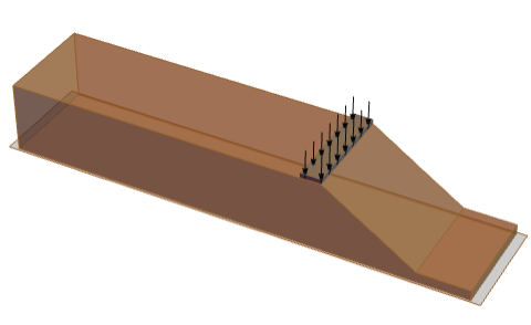
3D representation of the soil with a sloped surface and a load applied near the slope crest.
Needs["NDSolve`FEM`"]The base of the model is assumed to be fixed, representing the contact with the underlying ground not depicted in the figure. The left boundary is positioned far enough from the slope to remain unaffected by its deformation, effectively modeling an extension of the surrounding terrain. To limit computational cost, only the portion shown is simulated, with a vertical sliding boundary condition applied to the left face, allowing vertical movement while restricting horizontal displacement. Although such a condition can influence the slope response if the domain is too narrow, this is not the case here.
Similarly, the bottom-right region is constrained to move only vertically under the load transmitted by the sloped section, while horizontal motion is restricted due to the confining effect of adjacent ground. The soil mass is substantial, and given the clay-like properties of the material, self-weight effects are also considered as an additional mechanical load acting on the slope.
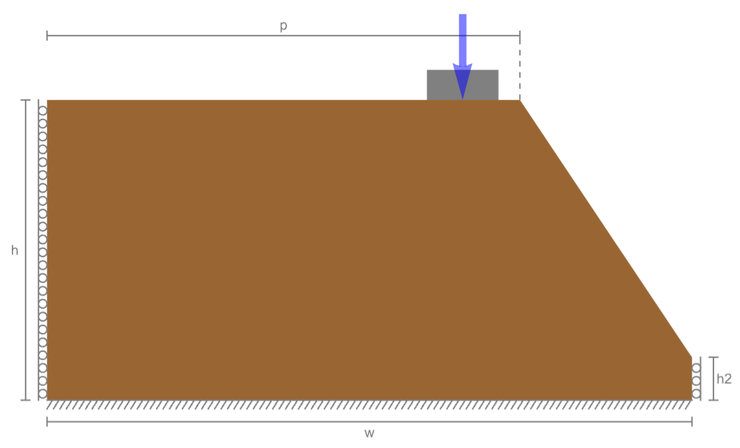
A two-dimensional view of the soil. The bottom boundary is fixed, and the lateral boundaries are constrained to move only in the vertical direction. The load is applied near the crest.
In the following, the geometrical features are defined, and the domain is meshed, with particular attention to areas expected to experience high stress and thus be involved in the plastic analysis.
l = 10;
h = 14;
w = 40;
h2 = 2;
p = w - 18;
It is worth noting that, given the dimensions of the top and bottom bases and the overall height, the geometry could also be represented as a 2D polygon and meshed with a uniform boundary grid. However, the loading configuration indicates that the vertical load and the sloped face are the primary sources of high stress concentrations and potential plastic zones. For this reason, a nonuniform mesh is adopted.
Each polygon edge is first discretized into a sequence of points with a specified minimum spatial resolution. This can be efficiently achieved using the ToGradedMesh function, which maps each segment into a graded distribution of points. The polygon is thus represented by a denser set of boundary nodes in critical regions. The final mesh is then generated by imposing an element size distribution that follows the graded boundary spacing, ensuring finer resolution where higher stress gradients are expected.
pts = {{0, 0}, {w, 0}, {w, h2}, {p, h}, {0, h}};sides = Partition[pts, 2, 1]mapPointsOnASide[side_, align_] := Module[{len, mesh, map},
len = Norm[Differences[side]];
mesh = ToGradedMesh[Line[{{0}, {len}}], <|"Alignment" -> align, "ElementCount" -> len|>, "MeshOrder" -> 1];
map = Flatten[mesh["Coordinates"]] / len;
(side[[1]] - # (Subtract@@side))& /@ map
]As mentioned earlier, the top and bottom sides require higher mesh resolution near the right boundary, while the sloped face demands finer discretization toward its ends to better capture stress gradients. In contrast, the left boundary does not require special refinement; its resolution is automatically determined during the meshing process once the full polygonal domain is generated.
mapTypes = {"Right", "Uniform", "BothEnds", "Left"};refinePolygon[sides_, mapTypes_] := DeleteDuplicates[Join@@MapThread[mapPointsOnASide, {sides, mapTypes}]]ptsRefined = refinePolygon[sides, mapTypes];dists = Norm /@ Differences[ptsRefined];colors = ColorData[{"DarkRainbow", "Reverse"}][#]& /@ Rescale[dists];Legended[Graphics[{FaceForm[LightGray], Polygon[pts], Thread[{colors, Thread[Point[Rest[ptsRefined]]]}]}, ImageSize -> Medium],
BarLegend[{{"DarkRainbow", "Reverse"}, MinMax[dists]}]]mesh = ToElementMesh[Polygon[ptsRefined], "MaxCellMeasure" -> 1.5]mesh["Wireframe"]It should be noted that the primary purpose of the graded mesh is twofold: to ensure high resolution in critical regions while keeping the total number of elements limited, thereby reducing computational cost. This aspect is particularly important for elasto-plastic analyses, which require multiple nonlinear iterations and significantly longer solving times compared to purely elastic simulations.
Soil Behavior
The material considered is a clay-like soil, which is prone to the formation of high shear zones that can lead to plasticization and potential sliding. However, its cohesive properties contribute to resisting deformation and delaying failure by increasing shear strength. The Drucker–Prager and Mohr–Coulomb yield criteria have both shown good capability in representing this type of soil behavior. In the following analysis, the Drucker–Prager model is adopted. It is worth noting, and will be discussed later, that under specific assumptions, these two criteria can be considered equivalent and compared by properly scaling their parameters.
vars = {{u[x, y], v[x, y], 0}, {x, y, z}};To solve the elasto-plastic problem, an initial purely elastic analysis is first performed using the defined material parameters and boundary conditions. The resulting elastic stress and strain fields serve as the initial approximation for the subsequent elasto-plastic solution, which is obtained by iteratively solving the same governing equations while incorporating the plasticity model.
pars = <|"YoungModulus" -> 50 * 10^6, "PoissonRatio" -> 0.45, "Thickness" -> l, "SolidMechanicsModelForm" -> "ExtendedPlaneStrain",
"MassDensity" -> 1800, "BodyLoadValue" -> {0, -9.81}|>;load = 0.55 * 10^7;The external load is applied on the top surface, near the sloped face. Since the governing equations will be solved multiple times, an auxiliary function is defined to handle not only the material parameters and problem variables but also the geometric domain and the loaded region. This modular approach allows the automatic generation of the corresponding PDEs while accommodating changes in domain properties or load configuration.
loadPos = x >= 19 && x <= 22 && y == heqn[vars_, pars_, mesh_, pos_, load_] :=
Module[{xLeft, xRight},
{xLeft, xRight} = First[mesh["Bounds"]];
{SolidMechanicsPDEComponent[vars, pars] == SolidBoundaryLoadValue[pos, vars, pars, <|"Force" -> {None, -load}|>],
SolidDisplacementCondition[(x == xLeft) || (x == xRight), vars, pars, <|"Displacement" -> {0, None}|>],
SolidFixedCondition[y == 0, vars, pars]}
]elasticDispl = NDSolveValue[eqn[vars, pars, mesh, loadPos, load], vars[[1]], {x, y}∈mesh];Show[mesh[...], ElementMeshDeformation[mesh, Most[elasticDispl], "ScalingFactor" -> 50][...]]The deformation results show a settlement of the top surface caused by both the self-weight of the soil and the applied external load. Before proceeding with the elasto-plastic analysis, the yield criterion can be evaluated based on the current stress state.
strain = SolidMechanicsStrain[vars, pars, elasticDispl];
stress = SolidMechanicsStress[vars, pars, strain];
The evaluation of the yield criterion requires computing the first stress invariant ![]() and the square root of the second invariant of the deviatoric stress,
and the square root of the second invariant of the deviatoric stress, ![]() . These quantities provide insight into the proximity of the material to yielding, as defined by the Drucker–Prager criterion. Further details can be found in the Drucker-Prager section in the Plasticity monograph.
. These quantities provide insight into the proximity of the material to yielding, as defined by the Drucker–Prager criterion. Further details can be found in the Drucker-Prager section in the Plasticity monograph.
vm = VonMisesStress[vars, pars, stress];
J2Sqrt = vm / Sqrt[3];I1 = Tr[stress];For stiff clay-like soils, the Drucker–Prager (DP) parameters indicate a cohesion parameter ![]() greater than zero and a noticeable level of pressure sensitivity
greater than zero and a noticeable level of pressure sensitivity ![]() [Rafiei, 2020].
[Rafiei, 2020].
αDP = 1 / 5;
kDP = 36000;yieldDP = J2Sqrt + αDP * I1 / 3 - kDP;RegionPlot[{yieldDP >= 0, yieldDP < 0}, {x, y}∈mesh, ...]As shown in the stress plot, the region near the toe of the slope experiences elevated stress levels that exceed the yield limit. Therefore, an elasto-plastic analysis is required to accurately predict the final deformation and stress redistribution within the soil mass.
setMaterialParameters[pars_, k_, α_] := Module[{parsPlastic},
	parsPlastic = pars;
	parsPlastic["CohesionParameter"] = k;
	parsPlastic["PressureSensitivity"] = α;
	parsPlastic["Plasticity"] = <|"YieldCriterion" -> "DruckerPrager"|>;
	parsPlastic
]parsPlastic = setMaterialParameters[pars, kDP, αDP];maxIteration = 100;elastoplasticDispl = elasticDispl;
updatePars = PDEModels`InitializePlasticity[vars, parsPlastic, elastoplasticDispl];
Monitor[
i = 1;
While[PDEModels`PlasticStepQ[vars, updatePars] && i < maxIteration,
updatePars = PDEModels`PlasticStrainStep[vars, updatePars, elastoplasticDispl];
elastoplasticDispl = NDSolveValue[eqn[vars, updatePars, mesh, loadPos, load], vars[[1]], {x, y}∈mesh];
i++;],
i]PDEModels`PlasticError[vars, updatePars]When simulations run for a long time, it may make sense to store the obtained results to hard disk such that they are readily available later without rerunning the simulation.
(*Export["elastoplasticDispl.mx", elastoplasticDispl]*)(*Import["elastoplasticDispl.mx"]*)Row[{Show[
mesh[...],
ElementMeshDeformation[mesh, elasticDispl[[1 ;; 2]], "ScalingFactor" -> 20][...],
ElementMeshDeformation[mesh, elastoplasticDispl[[1 ;; 2]], "ScalingFactor" -> 20][...], ...],
SwatchLegend[{LightGray, Blue, Red}, {"Undeformed", "Elastic", "Elastoplastic"}]}]The elasto-plastic solution shows a pronounced settlement in the loaded area. This behavior results from plasticization, which redistributes part of the load from the vertical direction into horizontal shear, causing a slight displacement of the sloped face toward the right. However, this horizontal shift remains limited and does not yet indicate a critical risk of slope failure. The potential for failure will be analyzed later; first, by examining the principal stress directions, it is possible to identify the likely orientation of the critical plane that could initiate and propagate a failure mechanism within the slope.
strainEP = SolidMechanicsStrain[vars, updatePars, elastoplasticDispl];
stressEP = SolidMechanicsStress[vars, updatePars, strainEP];{{σ1, σ2, σ3}, directions} = PDEModels`PrincipalEigensystem[vars, updatePars, stressEP];{e1, e2, e3} = directions[[All, 1 ;; 2]];MinMax[Head[σ1]["ValuesOnGrid"]]MinMax[Head[σ3]["ValuesOnGrid"]]Before proceeding with the discussion, it is useful to clarify an important notation convention. In solid mechanics, tensile stresses are typically considered positive and compressive stresses negative, as shown in the Solid Mechanics monograph. However, in soil mechanics, the convention is reversed: compressive stresses are often taken as positive since they are the most relevant.
Here the standard convention is used, where the positive value represents a tensile stress. That is why in the following compression plot the scale is negative.
Furthermore, principal stresses are ordered from the largest, ![]() , to the smallest,
, to the smallest, ![]() . Consequently, in soil mechanics applications, greater attention is often given to the third principal stress, since a higher compressive magnitude, i.e. a larger positive value under the soil convention, represents a critical stress condition for the material.
. Consequently, in soil mechanics applications, greater attention is often given to the third principal stress, since a higher compressive magnitude, i.e. a larger positive value under the soil convention, represents a critical stress condition for the material.
Legended[StreamPlot[e3, {x, y}∈mesh, ...], BarLegend[...]]Legended[StreamPlot[e1, {x, y}∈mesh, ...], BarLegend[...]]The Drucker–Prager and Mohr–Coulomb criteria describe soil yielding as governed by a combination of shear stress and mean normal stress. These models account for the influence of confinement and friction between soil particles. Failure occurs when the shear stress acting on a plane reaches a critical value determined by the material’s cohesion and internal friction angle.
The potential failure planes correspond to orientations where the shear stress to normal stress ratio reaches its maximum, typically at angles related to the material’s friction angle. Along these planes, plastic yielding initiates, marking the onset of irreversible deformation and the development of shear bands in the soil mass.
The Drucker–Prager and Mohr–Coulomb parameters can be converted one to the other, as equivalent forms. To facilitate the analysis of the failure planes, it is more convenient to refer to the angle of internal friction ![]() of the Mohr–Coulomb model, since it directly governs their orientation. For additional details, refer to the Plasticity monograph.
of the Mohr–Coulomb model, since it directly governs their orientation. For additional details, refer to the Plasticity monograph.
α[ϕ_] := (2/Sqrt[3])(Sin[ϕ]/3 + Sin[ϕ])
k[c_, ϕ_] := (2/Sqrt[3])(c Sin[ϕ]/3 + Sin[ϕ]){c0, ϕ0} = SolveValues[{αDP == α[ϕs], kDP == k[cs, ϕs], 0 < ϕs < Pi / 2, cs > 0}, {cs, ϕs}][[1]]//NThe failure lines are modulated by the internal friction angle, which shifts their orientation relative to the maximum shear direction. While the maximum shear direction rise is 45° with respect to the line connecting the first and third principal stress directions, in this case the angle became ![]() .
.
ω = π / 4 - ϕ0 / 2;The failure criterion predicts two symmetric directions oriented at equal angles about the principal stress directions. The positive direction ![]() and the negative direction
and the negative direction ![]() are computed using a positive and negative sign for the angle
are computed using a positive and negative sign for the angle ![]() , respectively. The streamlines of these directions define the lines of potential failure.
, respectively. The streamlines of these directions define the lines of potential failure.
posDir = e1 Sin[ω] + e3 Cos[ω];
negDir = e1 Sin[-ω] + e3 Cos[-ω];τmax = ElementMeshInterpolation[mesh, Abs[(Head[σ3]["ValuesOnGrid"] - Head[σ1]["ValuesOnGrid"]/2)]];Show[
DensityPlot[τmax[x, y], {x, y}∈mesh, ...],
StreamPlot[posDir, {x, y}∈mesh, ...],
StreamPlot[negDir, {x, y}∈mesh, ...],
Rule[...]]Failure happens along the curved red lines in the high shear stress ![]() areas.
areas.
The failure lines are shown in blue and red and their opacity is scaled with respect to maximum shear stress ![]() . The red lines represent the classical sliding pattern typically observed in slope failures. The blue lines show the mechanically equivalent conjugate failure line that completes the pair of possible failure orientations predicted by the Drucker–Prager and Mohr–Coulomb models. Although both orientations satisfy the failure criterion mathematically, only one of them, the red one, is physically activated. This line cannot be determined a priori, but is selected by the physics of the problem, depending on the slope geometry, loading direction and boundary conditions.
. The red lines represent the classical sliding pattern typically observed in slope failures. The blue lines show the mechanically equivalent conjugate failure line that completes the pair of possible failure orientations predicted by the Drucker–Prager and Mohr–Coulomb models. Although both orientations satisfy the failure criterion mathematically, only one of them, the red one, is physically activated. This line cannot be determined a priori, but is selected by the physics of the problem, depending on the slope geometry, loading direction and boundary conditions.
The plot also highlights regions of high shear stress beneath the loaded region with whiter areas. Together with the curved red failure lines, these illustrate the characteristic rotational movement that develops along these paths during a slope sliding failure.
Slope Failure Zones
In slope and foundation stability analysis, different failure mechanisms can develop depending on geometry, loading and soil strength. Three slope failure modes will be investigated next. As will be seen, the previously computed solution is typical for a face failure. The naming will become apparent later. Furthermore the toe and Prandtl failure modes will be introduced and compared. Together, these mechanisms describe the range of possible failure modes in soils subjected to shear and compressive stresses.
In the following, the load position is varied to highlight different failure mechanisms. Before proceeding, all the components required to solve the elasto-plastic behavior of the soil are encapsulated in an auxiliary function.
elastoplasticDisplFace = elastoplasticDispl;To illustrate the different failure mechanisms, the load position is varied. Before proceeding, all the components required to solve the elasto-plastic behavior of the soil are encapsulated in an auxiliary function.
elastoplasticSlopeSolve[vars_, pars_, loadedPos_, load_, initialDispl_, mesh_, maxIter_] := Module[{elastoplasticDispl, updatePars},
	elastoplasticDispl = initialDispl;
	updatePars = PDEModels`InitializePlasticity[vars, pars, elastoplasticDispl];
	Monitor[
	i = 1;
	While[PDEModels`PlasticStepQ[vars, updatePars]  && i < maxIter,
	updatePars = PDEModels`PlasticStrainStep[vars, updatePars, elastoplasticDispl];
	elastoplasticDispl = NDSolveValue[eqn[vars, updatePars, mesh, loadedPos, load], vars[[1]], {x, y}∈mesh];
	i++;], i];
	{updatePars, elastoplasticDispl}
	]
In order to investigate a different failure mechanism, the load position is changed while keeping the geometry and material properties unchanged.
loadPos2 = x >= 12 && x <= 15 && y == h;elasticDisplToe = NDSolveValue[eqn[vars, pars, mesh, loadPos2, load], vars[[1]], {x, y}∈mesh];{updateParsToe, elastoplasticDisplToe} = elastoplasticSlopeSolve[vars, parsPlastic, loadPos2, load, elasticDisplToe, mesh, maxIteration];Row[{ContourPlot[elastoplasticDisplFace[[1]], {x, y}∈mesh, PlotLegends -> False, PlotRange -> {All, {All, 17}}, AspectRatio -> Automatic, ContourStyle -> None, FrameTicks -> {Automatic, None}, ImageSize -> Medium, ColorFunction -> (ColorData["TemperatureMap"][Rescale[#1, {0., dmax = 0.018}]]&), ColorFunctionScaling -> False, Frame -> {True, True, False, False}, PlotLabel -> "Face failure", Epilog -> {Arrowheads[0.02], Table[Arrow[{{x, 14 + 2}, {x, 14}}], {x, 19, 22, 0.7}]}],
ContourPlot[elasticDisplToe[[1]], {x, y}∈mesh, PlotLegends -> Placed[Automatic, Right], ...]}]The plot highlights two distinct failure mechanisms. The first shows a more localized displacement concentrated near the upper part of the slope, gradually decreasing toward the base. In contrast, the second mechanism exhibits a broader zone of deformation, with a lower peak displacement but a wider affected area, particularly extending from the slope base.
To better highlight the difference between the two failures, the horizontal displacement is extracted along the sloped edge.
line[s_] := {p, h} + s ({w, h2} - {p, h})Plot[{Head[elastoplasticDisplFace[[1]]]@@line[s], Head[elastoplasticDisplToe[[1]]]@@line[s]}, {s, 0, 1}, ...
]The plot shows that the horizontal displacement of the slope, directed toward the sliding side, is greater in the face failure, where the load is applied close to the exposed slope face. In this mechanism, the face itself tends to collapse outward, hence the name face failure. By contrast, toe failure is characterized by movement concentrated in the lower part of the slope, where the failure surface emerges at the bottom section, known as the toe of the slope. In the plot, the effect of face failure is most pronounced near the crest, at point A, while at the base, point B, the displacement values are similar because they are constrained by the external boundary.
Both face and toe failures are types of sliding mechanisms associated with slope instability. Another form of soil failure is the Prandtl failure, which is instead related to the classical settlement behavior of the soil under loading. To observe this effect, the load must be positioned sufficiently far from the slope. This can be achieved by extending the right side of the domain while maintaining the same slope angle.
w = 60;
p = w - 18;pts = {{0, 0}, {w, 0}, {w, 2}, {p, h}, {0, h}};
sides = Partition[pts, 2, 1];ptsRefined = refinePolygon[sides, mapTypes];meshPrandtl = ToElementMesh[Polygon[ptsRefined], "MaxCellMeasure" -> 1.6]meshPrandtl["Wireframe"]loadPos3 = x >= 1 && x <= 4 && y == h;elasticDisplPrandtl = NDSolveValue[eqn[vars, pars, meshPrandtl, loadPos3, load], vars[[1]], {x, y}∈meshPrandtl];{updateParsPrandtl, elastoplasticDisplPrandtl} = elastoplasticSlopeSolve[vars, parsPlastic, loadPos3, load, elasticDisplPrandtl, meshPrandtl, maxIteration];Grid[{{
ContourPlot[Sqrt[Total[elastoplasticDisplFace^2]], {x, y}∈mesh, ...], ContourPlot[Sqrt[Total[elastoplasticDisplToe^2]], {x, y}∈mesh, ...]}, {
ContourPlot[Sqrt[Total[elastoplasticDisplPrandtl^2]], {x, y}∈meshPrandtl, ...], BarLegend[...]}}]Face failure occurs when the slip surface originates near the slope face and extends outward, leading to a shallow, progressive sliding of the surface material. Toe failure develops when the failure surface passes through or just beneath the slope toe, typically involving deeper soil layers and resulting in larger displacements. Prandtl failure, on the other hand, represents a classical plastic mechanism observed beneath loaded areas such as footings, characterized by a symmetrical fan-shaped pattern of shear zones connecting to the surface, not shown here.
The failure mechanism can also be interpreted from the failure lines. For this geometry, the negative failure direction ![]() , obtained using
, obtained using ![]() , is sufficient to represent the expected failure orientation. Furthermore, when scaled by the maximum shear stress, these lines directly illustrate the predicted failure pattern.
, is sufficient to represent the expected failure orientation. Furthermore, when scaled by the maximum shear stress, these lines directly illustrate the predicted failure pattern.
computeFailureLines[vars_, pars_, displ_, mesh_, ω_] := Module[{strainEP, stressEP, σ1, σ2, σ3, directions, e1, e2, e3, nNeg, τmax, pStrain},
strainEP = SolidMechanicsStrain[vars, pars, displ];
stressEP = SolidMechanicsStress[vars, pars, strainEP];
{{σ1, σ2, σ3}, directions} = PDEModels`PrincipalEigensystem[vars, pars, stressEP];
{e1, e2, e3} = directions[[All, 1 ;; 2]];
nNeg = e1 Sin[-ω] + e3 Cos[-ω];
τmax = ElementMeshInterpolation[mesh, Abs[(Head[σ3]["ValuesOnGrid"] - Head[σ1]["ValuesOnGrid"]/2)]];
{nNeg, τmax}
]{negDirToe, τmaxToe} = computeFailureLines[vars, updateParsToe, elastoplasticDisplToe, mesh, ω];{negDirPrandtl, τmaxPrandtl} = computeFailureLines[vars, updateParsPrandtl, elastoplasticDisplPrandtl, meshPrandtl, ω];Row[{Show[DensityPlot[τmax[x, y], {x, y}∈mesh, ...], StreamPlot[negDir, {x, y}∈mesh, ...], Rule[...]],
Show[DensityPlot[τmaxToe[x, y], {x, y}∈mesh, ...],
StreamPlot[negDirToe, {x, y}∈mesh, ...], Rule[...]],
Show[DensityPlot[τmaxPrandtl[x, y], {x, y}∈meshPrandtl, ...], StreamPlot[negDirPrandtl, {x, y}∈meshPrandtl, ...], Rule[...]]}]The failure lines are represented in black, and their opacity is scaled with respect to the maximum shear stress value ![]() . In all cases, the failure lines originate from the loaded region. Face and toe failure mechanisms exhibit similar patterns, but in the toe failure the mechanism is shifted away from the slope face, producing an indirect effect by pushing into the lower part of the slope. In contrast, the Prandtl failure is largely confined to the loaded area. Although some failure lines remain visible near the slope face due to the self-weight of the soil, the maximum shear intensity there is very low, indicating that collapse in that region is unlikely.
. In all cases, the failure lines originate from the loaded region. Face and toe failure mechanisms exhibit similar patterns, but in the toe failure the mechanism is shifted away from the slope face, producing an indirect effect by pushing into the lower part of the slope. In contrast, the Prandtl failure is largely confined to the loaded area. Although some failure lines remain visible near the slope face due to the self-weight of the soil, the maximum shear intensity there is very low, indicating that collapse in that region is unlikely.
As previously introduced, there is a clear distinction between the different soil failure mechanisms, most of which arise from the geometrical configuration of the slope. Due to the combined effects of external loading, self-weight and domain geometry, the slope may fail through face failure, where displacement is concentrated near the slope crest, or through toe failure, where a large portion of the soil mass begins to move from the slope base, dragging the entire slope with it.
The Prandtl-type failure, on the other hand, is characterized by a localized plasticization of the soil, leading to increased displacement compared to a purely elastic model. It primarily represents a settlement-type mechanism rather than a slope instability.
It is also worth noting that the general magnitude of displacement remains comparable across all configurations, which is mainly associated with the vertical component. While the externally loaded zone undergoes movement, the effect of the soil’s self-weight remains constant across the three geometries, producing a compressive state that can contribute to slope collapse under critical conditions.
Shear Strength Reduction
To compute a factor of safety for slope stability, the shear strength reduction method is commonly employed [Rafiei, 2020]. In this approach, the soil’s plasticity parameters are gradually reduced by a strength reduction factor, ![]() , until the model reaches failure. The value of
, until the model reaches failure. The value of ![]() at which numerical instability occurs represents the safety factor of the slope.
at which numerical instability occurs represents the safety factor of the slope.
To provide a clearer physical interpretation of the parameters involved, it is preferable to discuss them within the Mohr–Coulomb framework, since the corresponding conversion from the Drucker–Prager formulation has already been introduced. The two key parameters are the cohesion parameter ![]() , and the angle of internal friction
, and the angle of internal friction ![]() , which together define the shear strength of the soil. They determine the maximum admissible shear stress
, which together define the shear strength of the soil. They determine the maximum admissible shear stress ![]() that the soil can sustain for a given normal stress
that the soil can sustain for a given normal stress ![]() acting on a potential failure plane, expressed as
acting on a potential failure plane, expressed as ![]() .
.
τ[σ_, c_, ϕ_] := c + σ Tan[ϕ]σmax = Max[Abs@Head[σ3]["ValuesOnGrid"]]Plot[{τ[σ, c0, ϕ0], τ[σ, c0, 1.4 ϕ0], τ[σ, c0, 0.6ϕ0]}, {σ, 0, σmax}, ...]The shear strength reduction method progressively decreases the shear strength parameters by a reduction factor ![]() in order to determine how close the material is to its failure limit.
in order to determine how close the material is to its failure limit.
ϕ[F_] := ArcTan[Tan[ϕ0] / F]
c[F_] := c0 / FThe values for ![]() and
and ![]() have been computed above.
have been computed above.
In the following section, the shear strength reduction method is implemented. To simplify its application under different loading conditions and mesh configurations, all necessary procedures are wrapped in an auxiliary function. This function performs the following steps:
- Reduction of the Mohr–Coulomb parameters according to the specified reduction factor
 , and their conversion to the equivalent Drucker–Prager parameters.
Regarding the last step, in this case, the elasto-plastic solution is intentionally advanced toward numerical failure as the shear strength reduction method requires. However, due to the formulation of the elasto-plastic problem, convergence of the plastic flow may still be achieved even when the material is plastically yielding, resulting in a continuously increasing plastic strain. Although such a case does not represent numerical divergence, it leads to progressively larger displacements and an eventual loss of physical stability and meaning.
To account for this behavior, a tolerance threshold is introduced, based on the displacement error computed at the last iteration. The iterative displacement error, which can be extracted from the updated solution parameters, determines if the elasto-plastic computation is valid or not. While increasing the factor ![]() , the last valid iteration determines the factor of safety. To speed up the computation, a lower number of iterations is used.
, the last valid iteration determines the factor of safety. To speed up the computation, a lower number of iterations is used.
maxIteration = 50;maxDisplacementError = .5 10^-3;elastoplasticSlopeSolveAndCheck[vars_, pars_, loadPos_, load_, mesh_, maxIter_, maxError_] := Module[
{iterError, initialError, epDispl, updatePars, validQ = True},
epDispl = NDSolveValue[eqn[vars, pars, mesh, loadPos, load], vars[[1]], {x, y}∈mesh];
{updatePars, epDispl} = elastoplasticSlopeSolve[vars, pars, loadPos, load, epDispl, mesh, maxIter];
iterError = PDEModels`PlasticError[vars, updatePars];
If[iterError > maxError, validQ = False];
{updatePars, epDispl, validQ}
]shearStrengthReductionStep[vars_, pars_, loadPos_, load_, mesh_, maxIteration_, F_, maxError_] := Module[
{parsPlastic, elastoplasticDispl, updatePars, increaseFactorQ = True, kDP, αDP},
kDP = k[c[F], ϕ[F]];
αDP = α[ϕ[F]];
parsPlastic = setMaterialParameters[pars, kDP, αDP];
{updatePars, elastoplasticDispl, increaseFactorQ} = elastoplasticSlopeSolveAndCheck[vars, parsPlastic, loadPos, load, mesh, maxIteration, maxError];
{updatePars, elastoplasticDispl, increaseFactorQ}
]shearStrengthReduction[vars_, pars_, loadPos_, load_, mesh_, maxIteration_, maxError_, Fmin_, Fmax_] := Module[
{results, fPars, fDispl, increaseFactorQ},
results = Reap[Monitor[Do[
{fPars, fDispl, increaseFactorQ} = shearStrengthReductionStep[vars, pars, loadPos, load, mesh, maxIteration, F, maxError];
Sow[{F, fPars, fDispl}, "SSR"];
If[ !increaseFactorQ, Break[]];,
{F, Fmin, Fmax, 0.05}], "Factor: " <> ToString@F], "SSR"][[2, 1]];
Last@results
]Fmin = 1;
Fmax = 2;AbsoluteTiming[{fosF, fosPars, fosDispl} = shearStrengthReduction[vars, pars, loadPos, load, mesh, maxIteration, maxDisplacementError, Fmin, Fmax];]The loop terminates automatically once the solution no longer achieves convergence. The last step therefore corresponds to the maximum value of the reduction factor ![]() , which represents the factor of safety.
, which represents the factor of safety.
A factor of safety below 1 is not permissible, while in practice, higher factors of safety are required.
fosFplasticStrainFOS = PDEModels`PlasticStrain[vars, fosPars]equivalentPlasticStrainFOS = EquivalentStrain[vars, fosPars, plasticStrainFOS];ContourPlot[equivalentPlasticStrainFOS, {x, y}∈mesh, ...]The distribution of plastic strain shows that plasticization develops primarily along the slope, aligning with the characteristic failure surfaces associated with slope instability.
defMeshFosFirst = ElementMeshDeformation[mesh, elastoplasticDisplFace[[1 ;; 2]], "ScalingFactor" -> 20];
defMeshFosLast = ElementMeshDeformation[mesh, fosDispl[[1 ;; 2]], "ScalingFactor" -> 20];Show[mesh[...],
defMeshFosFirst[...],
defMeshFosLast[...], Rule[...]]The plot illustrates the deformation pattern at the final iteration of the shear strength reduction analysis, in red, showing a clear movement of the slope toward failure. The displacement at the crest is significantly higher than that observed with ![]() , obtained with the original material parameters, in blue.
, obtained with the original material parameters, in blue.
Slope Angle
As a final consideration, the inclination of the slope plays a fundamental role in stability analysis. The slope angle is one of the most significant geometric factors governing failure, and instability may occur solely due to the soil’s self-weight when the angle exceeds the material’s shear resistance.
In the following, the slope geometry is modified from its original inclination to four different slope angles, and for each configuration, the factor of safety is evaluated.
w = 50;
h2 = 2;
p = w - 18;delta = w - pθ = ArcTan[N@h / delta] / Degreeangles = {30, 40, 50, 60};deltas = N[h / Tan[# Degree]]& /@ anglesps = w - deltasgenerateSlopMesh[p_] := Module[{pts, sides, ptsRefined, mesh},
pts = {{0, 0}, {w, 0}, {w, 2}, {p, h}, {0, h}};
sides = Partition[pts, 2, 1];
ptsRefined = refinePolygon[sides, mapTypes];
mesh = ToElementMesh[Polygon[ptsRefined], "MaxCellMeasure" -> 2]
]meshes = generateSlopMesh[#]& /@ ps;#["Edgeframe"]& /@ meshesloadedPos = Table[x >= p - 3 && x <= p && y == h, {p, ps}];slopeAngleFOS = Monitor[MapThread[
shearStrengthReduction[vars, pars, #1, load, m = #2, maxIteration, maxDisplacementError, Fmin, Fmax]&, {loadedPos, meshes}], m["Edgeframe"]];fosAngleResult = slopeAngleFOS[[All, 1]]While all results indicate that the factor of safety is above 1, the last results are just barely above it.
BarChart[fosAngleResult, ChartLabels -> (ToString@#  <> "°" & /@ angles), PlotLabel -> "Factor of Safety", AxesLabel -> {"Slope
angle", "FOS"}]fosDisplacements = slopeAngleFOS[[All, 3]];fosDeformed = MapThread[ElementMeshDeformation[#1, #2[[1 ;; 2]], "ScalingFactor" -> 30]&, {meshes, fosDisplacements}];MapThread[Show[#1[...], #2[...], Rule[...]]&, {meshes, fosDeformed, fosAngleResult}]The factor of safety (FoS) decreases sharply as the slope angle increases. In particular, the last mesh, characterized by the steepest face, shows a very low value close to one, indicating almost no margin of stability. This is also confirmed by the deformed mesh, which clearly illustrates the progressive collapse of the slope. The failure is caused by the combined effect of several mechanisms: the self-weight of the soil compresses the material and induces a slight downslope movement; the external load further compresses the crest area, increasing the stress concentration in the underlying region; and finally, the accumulation of plastic strain needed to accommodate the extreme load leads to large displacements that drive the slope toward sliding and eventual failure.
3D Visualization
As a final step, since the example originates from a 3D slope geometry but is analyzed under plane strain conditions, it is possible to map the 2D deformation field onto the 3D model by assuming that the deformation remains constant along the embankment width.
m2D = ToElementMesh[Polygon[{{0, 0}, {w, 0}, {w, 2}, {ps[[-1]], h}, {0, h}}]];d2D = Last[fosDisplacements][[1 ;; 2]];m3D = ElementMeshRegionProduct[ToElementMesh[Line[{{-l}, {l}}]], m2D];
m3D = ElementMeshProjection[m3D, RotationTransform[-π / 2, {0, 0, 1}]];coords = m3D["Coordinates"];The displacement field can be mapped to three dimensions by assigning the planar ![]() coordinate to the 3D
coordinate to the 3D ![]() direction, and the planar
direction, and the planar ![]() coordinate to the 3D vertical
coordinate to the 3D vertical ![]() direction, while the 3D
direction, while the 3D ![]() direction remains constant with zero displacement.
direction remains constant with zero displacement.
displTransposed = {Head[d2D[[1]]]@@@coords[[All, {1, 3}]], ConstantArray[0., Length[coords]], Head[d2D[[2]]]@@@coords[[All, {1, 3}]]};diplsFun = ElementMeshInterpolation[m3D, #][x, y, z]& /@ displTransposed;To highlight the slope failure, several points along the sloped face are extracted to plot the displacement vectors. To achieve this, it is necessary to determine the equation of the plane representing the slope surface and then extract the points lying on that plane.
planeEq[x_] := h + (2 - h) / (w - ps[[-1]]) * (x - ps[[-1]]);onFace = Select[coords, Abs[#[[3]] - planeEq[#[[1]]]] < 10 ^ -6&];To achieve the desired effect of simulating the slope failure, the displacement field can be progressively scaled over several steps, generating a sequence of images that can be combined into an animation.
Monitor[imgs = Table[Rasterize@Show[
	P0 = {ps[[-1]] - 3, -l, h};
	dx = s  Head[#]@P0& /@ diplsFun;
Graphics3D[{Opacity[0.2], FaceForm[Black], Cuboid[P0 + dx, P0 + dx + {3, 2l, 1}], Opacity[.85], EdgeForm[], FaceForm[ColorData["SunsetColors"][0.15]], Cuboid[{w, -l, 0}, {w + 10, l, 2}]}], VectorDisplacementPlot3D[diplsFun, {x, y, z}∈m3D, ...], ViewPoint -> {20, -30, 20}, ...], {s, 0.05, 2.2, 0.05}];, s]ListAnimate[Join[imgs, Reverse@imgs]]The animation illustrates how the slope progressively reaches failure through sliding. Under the effect of the external load, the soil mass is compressed against the lower section, resulting in a horizontal displacement of the slope that evolves into a sliding failure. It should be noted that the final frames of the animation appear overly deformed due to the displacement scale factor applied to enhance visualization of where and how failure develops in the case with the steepest slope.
References
1. Chowdhury, R. (2009) Geotechnical Slope Analysis. ISBN: 978-1-135-19210-5. https://doi.org/10.1201/9780203864203.
2. Yang, G. (2025) "Ultimate Bearing Capacity of Embedded Strip Footings on Rock Slopes under Inclined Loading Conditions Using Adaptive Finite Element Limit Analysis." Scientific Reports, 15-1. https://doi.org/10.1038%2Fs41598-025-91234-2.
3. Rafiei, R. (2020) "Factor of Safety of Strain-Softening Slopes." Journal of Rock Mechanics and Geotechnical Engineering, 12-3. https://doi.org/10.1016/j.jrmge.2019.11.004.