Plasticity
| Contents | Theory of Small Strain Plasticity |
| Introduction | Load History |
| An Introductory Example | References |
Contents
Introduction
The notebook provides an early access to modeling plasticity in the Wolfram Language.
Plasticity refers to the ability of a solid to undergo permanent deformation, also known as plastic deformation when subjected to a load or deformation. Unlike elastic deformation, where a material returns to its original shape after the load is removed, plastic deformation involves a permanent change in shape.
Plasticity is a crucial concept in understanding the behavior of materials under various loading conditions, and it is essential in fields like structural engineering, materials science and manufacturing.
Materials that exhibit plastic behavior typically undergo a series of microscopic rearrangements or dislocation movements within their crystal structure when stressed beyond a certain threshold, known as the yield point. This phenomenon allows the material to remain deformed even after the applied stress is reduced. This type of material behavior is described by an elasto-plastic model, as it accounts for both the elastic and plastic components of deformation. It is often referred to simply as a plastic model for brevity.
Needs["NDSolve`FEM`"]An Introductory Example
To illustrate elasto-plastic behavior, a simple example is shown in the following. Consider a rectangular region representing a copper-like rod. With the left side fixed and a load applied on the right, this setup corresponds to the classical cantilever beam problem. In a first step, an elastic deformation is computed.
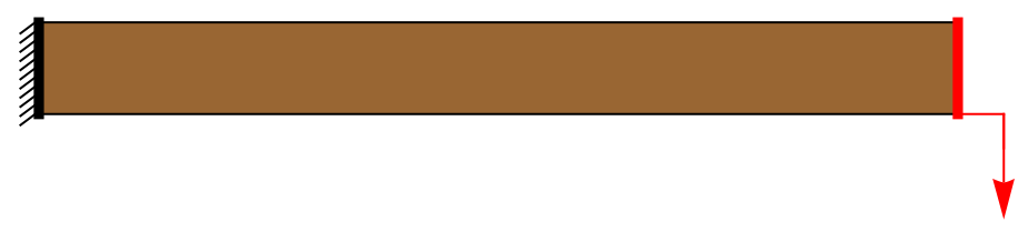
Geometry and boundary conditions of an initial elasto-plastic example. The left side is fixed, and a vertical displacement is applied on the right edge.
mesh = ToElementMesh[Rectangle[{0, 0}, {10, 1}], "MaxCellMeasure" -> 0.1];
mesh["Wireframe"]
Initially, the mechanical problem is solved assuming a fully elastic behavior. This solution serves as the starting point for the subsequent elasto-plastic computation. The next step is to define the material parameters and variables.
vars = {{u[x, y], v[x, y], 0}, {x, y, z}};pars = <|"YoungModulus" -> 90 * 10^9, "PoissonRatio" -> 0.3, "Thickness" -> 0.01, "SolidMechanicsModelForm" -> "ExtendedPlaneStrain"|>;eqn[vars_, pars_, imposedDispl_] := {SolidMechanicsPDEComponent[vars, pars] == {0, 0}, SolidFixedCondition[x == 0, vars, pars],
SolidDisplacementCondition[x == 10, vars, pars, <|"Displacement" -> {None, imposedDispl}|>]}δ = -1.15;elasticDispl = NDSolveValue[eqn[vars, pars, δ], vars[[1]], {x, y}∈mesh]Show[mesh["Wireframe"["MeshElement" -> "BoundaryElements"]], ElementMeshDeformation[mesh, elasticDispl[[1 ;; 2]], "ScalingFactor" -> 1]["Wireframe"[Rule[...]]]]After the elastic computation, it is important to evaluate the stress state. A material remains within the elastic regime as long as the stress does not exceed the yield stress, a material property. In other words, plastic deformation occurs when the material's yield stress, also called yielding point, is surpassed anywhere in the domain.
The von Mises plasticity criterion uses the von Mises stress measure to compute a stress value at a specific point in the domain. If at any point in the domain the stress value is beyond the yielding point, plastic deformation happens at that point.
strain = SolidMechanicsStrain[vars, pars, elasticDispl];
stress = SolidMechanicsStress[vars, pars, strain];
vm = Head@VonMisesStress[vars, pars, stress];ContourPlot[vm[x, y], {x, y}∈mesh, ...]For the purpose of this example, the material's yield stress is assumed to be reached at 650 [![]() ].
].
parsPlastic = pars;
parsPlastic["YieldStress"] = 650 * 10^6;Max[vm["ValuesOnGrid"]] >= parsPlastic["YieldStress"]Show[ContourPlot[vm[x, y], {x, y}∈mesh, ...],
ContourPlot[vm[x, y] == parsPlastic["YieldStress"], {x, y}∈mesh, ...]]The red dashed contour in the contour plot indicates where the von Mises stress exceeds the yield stress, suggesting that the material has gone beyond its elastic limit. This means that the assumption of elastic behavior is not justified. For an accurate result, plasticity effects must be taken into account.
RegionPlot[{vm[x, y] >= parsPlastic["YieldStress"], vm[x, y] < parsPlastic["YieldStress"]}, {x, y}∈mesh, ...]In the next step, a plastic analysis is performed. To do so, the "YieldStress" parameters need to be specified as above. The following then presents the typical solution loop used to incorporate plastic behavior.
To actually compute the nonlinear elasto-plastic behavior, the elastic displacement is needed, as it provides the initial estimate of the strain and stress fields. These fields are used to evaluate whether the material has reached the yield point. Once yielding is detected, a plastic correction is applied to adjust the stress state and update internal variables such as plastic strain.
maxIteration = 100;
elastoplasticDispl = elasticDispl;
updatePars = PDEModels`InitializePlasticity[vars, parsPlastic, elastoplasticDispl];
Monitor[
	i = 1;
	While[PDEModels`PlasticStepQ[vars, updatePars]  && i < maxIteration,
	updatePars = PDEModels`PlasticStrainStep[vars, updatePars, elastoplasticDispl];
	elastoplasticDispl = NDSolveValue[eqn[vars, updatePars, δ], vars[[1]], {x, y}∈mesh];
	i++;],
i]Legended[Show[
mesh[...],
ElementMeshDeformation[mesh, elasticDispl[[1 ;; 2]], "ScalingFactor" -> 1][...],
ElementMeshDeformation[mesh, elastoplasticDispl[[1 ;; 2]], "ScalingFactor" -> 1][...], Rule[...]],
SwatchLegend[{LightGray, Blue, Red}, {"Undeformed", "Elastic", "Elastoplastic"}]]There is a slight difference in the form of the deformed beam near the middle.
The final displacement is the result of two distinct contributions: elastic deformation and plastic deformation. The elastic component is reversible and recovers upon unloading, when the external constraints or loads are removed. The plastic deformation, however, represents a permanent change in the material’s shape, which will not be recovered once the object is unloaded.
strainEP = SolidMechanicsStrain[vars, updatePars, elastoplasticDispl];
stressEP = SolidMechanicsStress[vars, updatePars, strainEP];
vmEP = Head[VonMisesStress[vars, updatePars, stressEP]];
The SolidMechanicsStrain function returns the total strain, which is the sum of both the elastic and plastic components and possibly other strain components.
ContourPlot[vmEP[x, y], {x, y}∈mesh, ...]Note that the maximum stress is reduced due to the contribution of plastic strain in the elasto-plastic solution.
The maximum stress obtained with the elasto-plastic model is lower than that of the fully elastic one, due to plastic deformation redistributing stress and preventing further stress accumulation beyond the yield point.
Max[vmEP["ValuesOnGrid"]]Note that the maximum stress values obtained from the InterpolatingFunction may appear slightly higher than the specified yield stress. This effect arises from the implicit discretization in the finite element method.
Plot[{vmEP[x, 0], parsPlastic["YieldStress"]}, {x, 0, 1}, ...]This is a local artifact, typically occurring near a fixed boundary due to interpolation behavior.
RegionPlot[{vmEP[x, y] >= parsPlastic["YieldStress"], vmEP[x, y] <
	parsPlastic["YieldStress"]}, {x, y}∈mesh, ...]
The difference between the purely elastic and the elasto-plastic model can be observed directly in the stress-strain plot by evaluating stress and strain at point near the top-left corner. The point location is arbitrary.
{Px, Py} = {0.3, 0.98};σVME = vm[Px, Py]σVMEP = vmEP[Px, Py]Show[Plot[{updatePars["YieldStress"], ϵ * updatePars["YoungModulus"]}, {ϵ, 0, ϵf = 0.018}, PlotStyle -> {Dashed, Dashed}, ...],
ListLinePlot[{{0, 0}, {σVMEP / updatePars["YoungModulus"], σVMEP}, {ϵf, σVMEP}}],
ListPlot[{{{σVME / updatePars["YoungModulus"], σVME}}, {{σVME / updatePars["YoungModulus"], σVMEP}}}, ...], ListPlot[{{{updatePars["YieldStress"] / updatePars["YoungModulus"], updatePars["YieldStress"]}}}, ...]]In both the elastic and the elasto-plastic case, the final deformation, the amount of strain, remains the same. This is expected, as it is imposed by the displacement boundary conditions. However, the final stress state differs significantly. In the fully elastic model, the stress exceeds the yielding point. This is unrealistic because a material stressed beyond the yield point will deform permanently. The elasto-plastic model effectively captures perfect plasticity, characterized by continued deformation beyond the yield point while the stress remains constant at the yield limit.
Note that the material has a low elastic modulus and a low yielding point, resulting in a relatively high final deformation. This effect was created intentionally to emphasize the difference between a fully elastic model and an elasto-plastic model.
To visualize the plastic deformation only, one may proceed as follows:
plasticStrain = PDEModels`PlasticStrain[vars, updatePars]Computing the equivalent strain transforms the strain tensor into a single strain measure, in the same way that the von Mises stress converts the stress tensor into a single stress measure.
equivalentPlasticStrain = EquivalentStrain[vars, updatePars, plasticStrain]ContourPlot[equivalentPlasticStrain, {x, y}∈mesh, ...]The elasto-plastic model results in an accumulation of plastic strain. Regions where plastic strain develops are referred to as plasticized areas and correspond to the ones in red in the previous plot.
When solving the same PDE using pars or updatePars with no applied load, the elasto-plastic model retains the permanent deformation, whereas the linear elastic model fully recovers and shows no residual deformation. More information on the residual plastic strain can be found in the Permanent deformation section.
Theory of Small Strain Plasticity
Modeling an elasto-plastic material requires capturing how the material responds to both reversible and irreversible deformations. The reversible part corresponds to an elastic deformation, and the irreversible part represents an inelastic, permanent deformation. In the context of plasticity, the inelastic deformation is referred to as plastic strain. Plastic strain can be introduced through two common approaches: additive or multiplicative decomposition. The additive decomposition of strain is typically used in small strain, infinitesimal formulations, where the total strain is assumed to be the sum of elastic and plastic components. In contrast, for large deformation scenarios, a multiplicative decomposition of the deformation gradient is employed to more accurately capture the nonlinear behavior.
To keep things simple, the following description of plasticity starts from the infinitesimal strain case, where the total strain results from the symmetric gradient of the displacement:
For infinitesimal strain formulations, the additive decomposition expresses the total strain as the sum of elastic and inelastic components:
The stress is evaluated based exclusively on the elastic strain:
The elastic strain can be expressed as:
The inelastic strain is given by:
In this case there is a only plastic inelastic strain
To implement an elasto-plastic model, the plastic strain ![]() must be explicitly accounted for, just like a thermal strain, for example.
must be explicitly accounted for, just like a thermal strain, for example.
To express a plastic strain, an elasto-plastic model requires the following information:
Indeed, there is a actually a third possible requirement, a hardening model, but to keep things simple, that will be discussed later.
A yield function ![]() specifies where and at what value in a object one can expect to see plastic deformation. The yield function specifies when a material starts yielding. Typically, the yield function is defined such that for
specifies where and at what value in a object one can expect to see plastic deformation. The yield function specifies when a material starts yielding. Typically, the yield function is defined such that for ![]() there is no plastic deformation. This is typically the case when the stress at that specific point in the material is less then the yield stress value of the material. A point without plastic deformation is described by an elastic modulus, just like in the standard linear elastic case. When there is no plastic deformation in some part of the region, the plastic strain
there is no plastic deformation. This is typically the case when the stress at that specific point in the material is less then the yield stress value of the material. A point without plastic deformation is described by an elastic modulus, just like in the standard linear elastic case. When there is no plastic deformation in some part of the region, the plastic strain ![]() .
.
Once the yield function reaches ![]() at a point in the material, there is plastic behavior at that point and a flow rule governs how plastic strain evolves there. It is common that a material has reached the yielding limit at some points in the material and not at others. Note that once
at a point in the material, there is plastic behavior at that point and a flow rule governs how plastic strain evolves there. It is common that a material has reached the yielding limit at some points in the material and not at others. Note that once ![]() is reached at a point, the elastic strain
is reached at a point, the elastic strain ![]() no longer increases but the plastic strain
no longer increases but the plastic strain ![]() will, and thus the total strain
will, and thus the total strain ![]() also has to increase.
also has to increase.
The process of computing the plastic strain involves a two-step approach: first, an elastic solution is computed. This will typically overshoot, and then a plastic correction is applied to make sure the elastic strain does not increase but the plastic strain does. This then obtains the elasto-plastic solution.

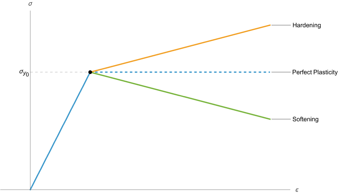
Strain and stress beyond the yield limit.
Keep in mind that only an increase in elastic strain has an increase in stress as a result. So once the material reaches its yield stress, it continues to deform plastically without any further increase in stress. The curve after the yield limit is horizontal, and this behavior is known as a perfect plasticity. Should that curve not be horizontal, then a hardening model will need to be used, as explained later.
The process is laid out in more detail in the following sections.
Yield Function
The yield function ![]() defines the conditions that determine the onset of plastic deformation in the material and is a function of the stress
defines the conditions that determine the onset of plastic deformation in the material and is a function of the stress ![]() and the yield stress material property
and the yield stress material property ![]() . For instance, the introductory example is based on the von Mises yield function, which reads:
. For instance, the introductory example is based on the von Mises yield function, which reads:
Here ![]() is the von Mises stress measure employed and thus named the von Mises yield criterion.
is the von Mises stress measure employed and thus named the von Mises yield criterion.
The yield function ![]() defines different regions in a body under load. A region where
defines different regions in a body under load. A region where ![]() corresponds to an elasticity region. Here the material is fully elastic. The surface where
corresponds to an elasticity region. Here the material is fully elastic. The surface where ![]() represents the onset of plasticity. On this surface, there is plastic deformation.
represents the onset of plasticity. On this surface, there is plastic deformation.

The von Mises stress in a beam under load. The red dashed contour represents the onset of plasticity ![]() .
.
An important point is that by definition, the region where ![]() is inadmissible because it represents stress levels that are not physically attainable.
is inadmissible because it represents stress levels that are not physically attainable.

The von Mises stress in a beam under load. The red area represents the regions where the von Mises stress is beyond the yield limit ![]() . Here plastic deformation needs to be considered.
. Here plastic deformation needs to be considered.
In plasticity theory, various yield criteria are used, each defined by a different yield function. The choice of criterion depends on the material’s mechanical behavior and the loading conditions and is often guided by the dominant stress state and experimental calibration based on the failure criterion.
At least an initial yield stress ![]() is used in yield functions because it represents the stress level where plasticity starts. It is a property of the material that needs to be found from experimental measurements or literature data.
is used in yield functions because it represents the stress level where plasticity starts. It is a property of the material that needs to be found from experimental measurements or literature data.
In addition, since stress is a tensor quantity, it is generally referred to as a stress state rather than a stress level, implicitly acknowledging that a yield function is used to evaluate this stress in relation to a material’s yield limit. The yield function itself is a scalar-valued function that transforms the multi-component stress tensor into a scalar measure. Depending on the chosen yield function, it can depend on different measures of stress. For example, the von Mises yield function reduces the stress tensor to the von Mises stress, a scalar value. In such cases, it becomes appropriate to refer to the stress level, since the tensor has been mapped to a scalar quantity suitable for comparison against the yield stress.
The Wolfram Language provides some predefined yield criteria that are specified through the "YieldCriterion" in a "Plasticity" association in pars, shown later. At the same time, a general purpose yield function can be set up.
von Mises yield criterion
The von Mises yield criterion is widely used for ductile material, and it is based on the concept that yielding occurs when the von Mises stress ![]() measure exceeds the critical value of initial yield stress
measure exceeds the critical value of initial yield stress ![]() .
.
Written out in component form:
Equivalently, the von Mises yield criterion can be expressed in terms of the principal stress as:
The introductory example made use of the von Mises yield criterion. The von Mises yield criterion is the default yield criterion. To set the yield criterion, the "YieldCriterion" needs to be set in the parameters pars.
pars["Plasticity"] = <|"YieldCriterion" -> "VonMises"|>;Tresca yield criterion
The Tresca criterion is suitable for materials prone to shear failures, such as the majority of brittle materials. It is based on the maximum shear stress, and the yield function reads:
where ![]() is the shear yield stress, a material property that must be specified, and
is the shear yield stress, a material property that must be specified, and ![]() are the principal stresses, the eigenvalues of the stress tensor.
are the principal stresses, the eigenvalues of the stress tensor.
pars["Plasticity"] = <|"YieldCriterion" -> "Tresca"|>;pars["ShearYieldStress"] = τy0;Depending on the material characterization, the yield shear stress ![]() can be related to the uniaxial yield stress
can be related to the uniaxial yield stress ![]() by reducing the Tresca criterion to a uniaxial stress state
by reducing the Tresca criterion to a uniaxial stress state ![]() ,
, ![]() and
and ![]() . At yield, where
. At yield, where ![]() , the criterion gives:
, the criterion gives:
The Tresca criterion states that yielding begins when the maximum shear stress, equal to half the difference between the largest and smallest principal stresses, reaches a critical value.
In the following example, the same loading scheme used for the introductory beam example is adopted, but the Tresca yield criterion is applied to evaluate the elasto-plastic response.
vars = {{u[x, y], v[x, y], 0}, {x, y, z}};
pars = <|"YoungModulus" -> 90 * 10^9, "PoissonRatio" -> 0.3, "Thickness" -> 0.01, "SolidMechanicsModelForm" -> "ExtendedPlaneStrain"|>;
mesh = ToElementMesh[Rectangle[{0, 0}, {10, 1}], "MaxCellMeasure" -> 0.1];eqn[vars_, pars_, imposedDispl_] := {SolidMechanicsPDEComponent[vars, pars] == {0, 0}, SolidFixedCondition[x == 0, vars, pars],
SolidDisplacementCondition[x == 10, vars, pars, <|"Displacement" -> {None, imposedDispl}|>]}δ = -1.15;elasticDispl = NDSolveValue[eqn[vars, pars, δ], vars[[1]], {x, y}∈mesh];Show[mesh["Wireframe"["MeshElement" -> "BoundaryElements"]], ElementMeshDeformation[mesh, elasticDispl[[1 ;; 2]], "ScalingFactor" -> 1][...]]strain = SolidMechanicsStrain[vars, pars, elasticDispl];
stress = SolidMechanicsStress[vars, pars, strain];The Tresca criterion states that yielding begins when the maximum shear stress, equal to half the difference between the largest and smallest principal stresses, reaches a critical value.
parsPlastic = pars;
parsPlastic["ShearYieldStress"] = 325 * 10^6;parsPlastic["Plasticity"] = <|"YieldCriterion" -> "Tresca"|>;tresca = (1/2)Max[Abs[Subtract@@#]& /@ Subsets[{σ1, σ2, σ3}, {2}]]{principalStress, pricipalStressDirections} = PDEModels`PrincipalEigensystem[vars, pars, stress];trescaStress = tresca /. Thread[Rule[{σ1, σ2, σ3}, principalStress]];RegionPlot[{trescaStress >= parsPlastic["ShearYieldStress"], trescaStress < parsPlastic["ShearYieldStress"]}, {x, y}∈mesh, ...]According to the Tresca criterion, the highest stress concentration occurs near the fixed support, tensile at the top side and compressive at the bottom side, leading to the formation of a plastic hinge, a region prone to significant permanent plastic deformation.
The difference between the Tresca and von Mises criteria becomes evident in stress states dominated by shear, with Tresca generally being slightly more conservative than von Mises. This can be visualized as follows:
vm = Head@VonMisesStress[vars, pars, stress];σY0 = 2 parsPlastic["ShearYieldStress"];RegionPlot[{vm[x, y] >= σY0, trescaStress >= parsPlastic["ShearYieldStress"]}, {x, y}∈mesh, Rule[...]]The Tresca criterion predicts a larger region beyond the elastic limit than von Mises, reflecting its more conservative nature, particularly in areas of high shear stress.
τ = stress[[1, 2]];DensityPlot[τ, {x, y}∈mesh, ...]In the next step, a plastic analysis is performed. To do so, the "ShearYieldStress" parameters need to specified as above. The following then presents the typical solution loop used to incorporate plastic behavior.
To actually compute the nonlinear elasto-plastic behavior, the elastic displacement is needed, as it provides the initial estimate of the strain and stress fields. Once yielding is detected, a plastic correction is applied to adjust the stress state and update internal variables such as plastic strain.
maxIteration = 150;
elastoplasticDispl = elasticDispl;
updatePars = PDEModels`InitializePlasticity[vars, parsPlastic, elastoplasticDispl];
Monitor[
	i = 1;
	While[PDEModels`PlasticStepQ[vars, updatePars]  && i < maxIteration,
	updatePars = PDEModels`PlasticStrainStep[vars, updatePars, elastoplasticDispl];
	elastoplasticDispl = NDSolveValue[eqn[vars, updatePars, δ], vars[[1]], {x, y}∈mesh];
	i++;],
	i]
When simulations run for a long time, it may make sense to store the obtained solution such that they are readily available later without rerunning the simulation. Both displacement and parameter data is required to carry out post-processing correctly.
(*Export["displacement.mx", elastoplasticDispl]*)
(*Export["parameters.mx", updatePars]*)(*Import["displacement.mx"]*)
(*Import["parameters.mx"]*)Legended[Show[
mesh[...],
ElementMeshDeformation[mesh, elasticDispl[[1 ;; 2]], "ScalingFactor" -> 1][...],
ElementMeshDeformation[mesh, elastoplasticDispl[[1 ;; 2]], "ScalingFactor" -> 1][...], Rule[...]]
, SwatchLegend[{LightGray, Blue, Red}, {"Undeformed", "Elastic", "Elastoplastic"}]]As for the introductory example, there is a slight difference in the form of the deformed beam near the middle.
The final displacement is the result of two distinct contributions: elastic deformation and plastic deformation. The elastic component is reversible and recovers upon unloading, when the external constraints or loads are removed. The plastic deformation, however, represents a permanent change in the material’s shape, which will not be recovered once the object is unloaded. The presence of the plastic strain alters the stress state found in the elasto-plastic solution, leading to a satisfaction of the Tresca criterion.
strainEP = SolidMechanicsStrain[vars, updatePars, elastoplasticDispl];
stressEP = SolidMechanicsStress[vars, updatePars, strainEP];
The SolidMechanicsStrain function returns the total strain, which is the sum of both the elastic and plastic components and possibly other strain components.
{{s1, s2, s3}, directions} = PDEModels`PrincipalEigensystem[vars, updatePars, stressEP];trescaStressEP = EvaluateOnElementMesh[{x, y}, tresca /. {σ1 -> s1, σ2 -> s2, σ3 -> s3}, mesh];The Tresca criterion is governed by the maximum shear stress, which derives from the largest difference between the principal stresses. This manifests in the principal stress directions, highlighting the potential failure planes, or lines in 2D. These planes correspond to the orientations of maximum shear stress where yielding is most likely to begin. They are crucial in elasto-plastic materials, as they define the onset and direction of plastic flow, marking the transition from elastic behavior to permanent deformation.
{e1, e2, e3} = directions[[All, 1 ;; 2]];In principal stress space, the axes are aligned with the principal stresses directions ![]() , while the failure planes, where the maximum shear stress acts, are oriented at 45° with respect to the line connecting the first and last principal stresses. They are defined as
, while the failure planes, where the maximum shear stress acts, are oriented at 45° with respect to the line connecting the first and last principal stresses. They are defined as ![]() and can be visualized as follows.
and can be visualized as follows.
np = (e1 - e3/Sqrt[2]);
nm = (e1 + e3/Sqrt[2]);Show[
ContourPlot[trescaStressEP[x, y], {x, y}∈mesh, ...],
StreamPlot[np, {x, y}∈mesh, ...],
StreamPlot[nm, {x, y}∈mesh, ...],
ImageSize -> Medium]The blue and green lines indicate the failure paths predicted by the criterion. These lines mark the regions where rupture is most likely to occur. The failure paths are particularly prominent near the fixed left side where shear stress is highest. These lines reflect the characteristic fracture patterns of brittle materials such as glass, rock or ceramics, which typically develop at about 45° to the loading direction. Similar diagonal cracks can often be seen in everyday situations, like across tiled floors, house walls or sidewalks under heavy load.
The failure paths are defined at 45° with respect to the lines connecting the first and last principal stress directions; they can be oriented either clockwise or counterclockwise. This is why two colors and two sets of lines are shown. From a practical perspective, there is no difference in choosing one orientation over the other; according to this criterion, both directions are equivalent in terms of failure probability.
Mohr-Coulomb yield criterion
The Mohr–Coulomb yield criterion is generally used for soil or granular materials. It states that yielding occurs when the shear stress on some plane reaches a critical value, which depends linearly on the normal stress acting on that plane. The critical yield shear stress can be expressed as a function of stress:
where ![]() is the normal stress acting on the reference plane, and
is the normal stress acting on the reference plane, and ![]() and
and ![]() are material parameters, respectively named Cohesion and Angle of internal friction.
are material parameters, respectively named Cohesion and Angle of internal friction.
In the general 3D case, where the stress ![]() is a 3×3 tensor, the expression of the criterion is:
is a 3×3 tensor, the expression of the criterion is:
where ![]() is the first stress invariant,
is the first stress invariant, ![]() is the second invariant of the deviatoric stress, and
is the second invariant of the deviatoric stress, and ![]() is the Lode angle related to the stress state, defined as:
is the Lode angle related to the stress state, defined as:
where the deviatoric operator is ![]() ,
,
where ![]() is the first stress invariant and
is the first stress invariant and ![]() is the second invariant of the deviatoric stress, respectively defined as:
is the second invariant of the deviatoric stress, respectively defined as:
where the deviatoric operator is ![]() .
.
The angle ![]() , known as the Lode angle, characterizes the stress state by quantifying the influence of each principal stress relative to the other principal stresses. It is defined as:
, known as the Lode angle, characterizes the stress state by quantifying the influence of each principal stress relative to the other principal stresses. It is defined as:
Due the presence of the second invariant of the deviatoric part of the stress tensor ![]() , this criterion is often reformulated as:
, this criterion is often reformulated as:
Here ![]() is known as the friction coefficient,
is known as the friction coefficient, ![]() as the cohesion intercept, and
as the cohesion intercept, and ![]() is the Lode angle dependency function.
is the Lode angle dependency function.
pars["Plasticity"] = <|"YieldCriterion" -> "MohrCoulomb"|>;pars["Cohesion"] = c;pars["AngleInternalFriction"] = ϕ;An example of the Mohr–Coulomb yield criterion is given in the Drucker–Prager yield criterion section.
Drucker-Prager yield criterion
The Drucker–Prager yield criterion is generally used for materials that exhibit pressure-dependent strength, such as soil or granular materials.
It is based on the deviatoric stress through the second stress invariants ![]() , with the yield function defined as:
, with the yield function defined as:
where ![]() is the first stress invariant, and αDP and kDP are material parameters known as Cohesion Parameter and Pressure Sensitivity.
is the first stress invariant, and αDP and kDP are material parameters known as Cohesion Parameter and Pressure Sensitivity.
The Drucker–Prager criterion is similar to the Mohr–Columb one but neglects the influence of ![]() . Moreover, their parameters can be related as:
. Moreover, their parameters can be related as:
where ![]() and
and ![]() are the material parameters of the Mohr–Coulomb criterion, and can be mapped using the relations:
are the material parameters of the Mohr–Coulomb criterion, and can be mapped using the relations:
The sign can be chosen as positive to match the tensile meridian or negative to match the compressive meridian of the Mohr–Coulomb's pyramid. These parameter names are similar to the one appearing in the compact Mohr–Coulomb, but they are different, ![]() and
and ![]() .
.
pars["Plasticity"] = <|"YieldCriterion" -> "DruckerPrager"|>;pars["CohesionParameter"] = k;pars["PressureSensitivity"] = α;In this example, the Mohr–Coulomb and Drucker–Prager yield criteria are compared through a classical problem in soil mechanics: the settlement of a strip footing constructed on clayey soil. The footing is subjected to a vertical load, and the soil response depends on its elasto-plastic behavior. To ensure the stability of the construction and to predict the expected settlement, the soil’s plastic response must be analyzed using appropriate yield criteria.
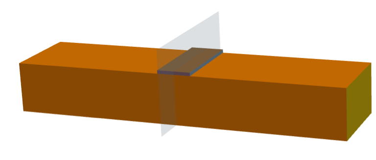
Soil portion of interest, brown, with a strip footing, gray. The transparent plane indicates the plane of symmetry.
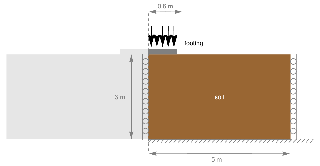
Equivalent planar load scheme. Thanks to the constant geometry along the footing direction, the problem can be reduced to a two-dimensional form. Exploiting symmetry with respect to the strip footing centerline, only the right half is modeled. A roller-like boundary condition is applied along the symmetry plane, left side, while a similar roller-like boundary condition is imposed on the right side to account for the surrounding soil, allowing only vertical displacements. The base is fixed, and the external load is applied on the top surface over the footing.
h = 3;
l = 5;
footing = 0.6;ϕMC = 30 Degree;
cMC = 30 10^3;A nonhomogeneous mesh is used to refine the discretization near the loaded zone, while employing a coarser mesh on the opposite side, which reduces the total number of elements without compromising accuracy in the critical region near the footing.
mesh = ElementMeshRegionProduct[ToGradedMesh[Line[{{0}, {l}}], <| "Alignment" -> "Left", "ElementCount" -> 8l|>], ToGradedMesh[Line[{{0}, {h}}], <| "Alignment" -> "Right", "ElementCount" -> 8h|>]];
mesh["Wireframe"]vars = {{u[x, y], v[x, y], 0}, {x, y, z}};pars = <|"YoungModulus" -> 50 * 10^6, "PoissonRatio" -> 0.45, "Thickness" -> l, "SolidMechanicsModelForm" -> "ExtendedPlaneStrain"|>;load = 1.52 * 10^6;eqn[vars_, pars_] := {SolidMechanicsPDEComponent[vars, pars] == SolidBoundaryLoadValue[x <= footing && y == h, vars, pars, <|"Force" -> {None, -load}|>],
SolidDisplacementCondition[x == 0 || x == l, vars, pars, <|"Displacement" -> {0, None}|>],
SolidDisplacementCondition[y == 0, vars, pars, <|"Displacement" -> {None, 0}|>]
}elasticDispl = NDSolveValue[eqn[vars, pars], vars[[1]], {x, y}∈mesh]Show[mesh[...], ElementMeshDeformation[mesh, elasticDispl[[1 ;; 2]], "ScalingFactor" -> 20][...]]strain = SolidMechanicsStrain[vars, pars, elasticDispl];
stress = SolidMechanicsStress[vars, pars, strain];The elastic solution for soil may not be sufficiently accurate once the material exceeds the yield limit. To address this, the Mohr–Coulomb and Drucker–Prager yield criteria are compared with the actual stress state. The Mohr–Coulomb criterion is simpler to express in compact form but requires reformulating the material parameters, whereas the Drucker–Prager formulation can directly adapt the parameters used in Mohr–Coulomb.
For visualization of the criteria, it is necessary to compute the first stress invariant ![]() , the square root of the second invariant of the deviatoric stress
, the square root of the second invariant of the deviatoric stress ![]() , and the Lode angle dependency function
, and the Lode angle dependency function ![]() . With these quantities, both yield surfaces can be represented and compared under the applied loading conditions.
. With these quantities, both yield surfaces can be represented and compared under the applied loading conditions.
αMC = Sin[ϕMC] / 3;
kMC = cMC Cos[ϕMC];αDP = (2/Sqrt[3])(Sin[ϕMC]/3 - Sin[ϕMC]);
kDP = (6/Sqrt[3])(cMC Cos[ϕMC]/3 - Sin[ϕMC]);I1 = Tr[stress];vm = VonMisesStress[vars, pars, stress];
J2Sqrt = vm / Sqrt[3];devS = stress - (1/3)Tr[stress] IdentityMatrix[3];arg = Clip[((Det[devS]/J2Sqrt^2))^3, {-1, 1}];
theta = (1/3)ArcCos[arg];
m = (1/Sqrt[3])(1 + Sin[ϕMC])Cos[theta] - (1 - Sin[ϕMC])Cos[theta + 2Pi / 3];mcCriterion = J2Sqrt m + αMC * I1 - kMC;dpCriterion = J2Sqrt + αDP * I1 / 3 - kDP;RegionPlot[{dpCriterion >= 0, mcCriterion >= 0, dpCriterion < 0 && mcCriterion < 0}, {x, y}∈mesh, ...]The Drucker–Prager criterion appears slightly more conservative than the Mohr–Coulomb one, and in both cases the soil beneath the footing is subjected to significant loading. Interestingly, the highest stresses do not occur directly under the footing but rather in deeper regions of the soil that extend up to the surface near the footing edge. This happens because those zones experience larger distortional shear deformations, whereas the area immediately below the footing is mainly under a pure compressive state.
Next, the material parameters are defined, and the elasto-plastic problem is solved using both yield criteria.
parsPlasticMC = pars;
parsPlasticMC["Cohesion"] = cMC;
parsPlasticMC["AngleInternalFriction"] = ϕMC;parsPlasticMC["Plasticity"] = <|"YieldCriterion" -> "MohrCoulomb"|>;maxIteration = 150;
elastoplasticDisplMC = elasticDispl;
updateParsMC = PDEModels`InitializePlasticity[vars, parsPlasticMC, elastoplasticDisplMC];
Monitor[
i = 1;
While[PDEModels`PlasticStepQ[vars, updateParsMC] && i < maxIteration,
updateParsMC = PDEModels`PlasticStrainStep[vars, updateParsMC, elastoplasticDisplMC];
elastoplasticDisplMC = NDSolveValue[eqn[vars, updateParsMC], vars[[1]], {x, y}∈mesh];
i++;],
i]parsPlasticDP = pars;
parsPlasticDP["CohesionParameter"] = kDP;
parsPlasticDP["PressureSensitivity"] = αDP;parsPlasticDP["Plasticity"] = <|"YieldCriterion" -> "DruckerPrager"|>;maxIteration = 150;
elastoplasticDisplDP = elasticDispl;
updateParsDP = PDEModels`InitializePlasticity[vars, parsPlasticDP, elastoplasticDisplDP];
Monitor[
i = 1;
While[PDEModels`PlasticStepQ[vars, updateParsDP] && i < maxIteration,
updateParsDP = PDEModels`PlasticStrainStep[vars, updateParsDP, elastoplasticDisplDP];
elastoplasticDisplDP = NDSolveValue[eqn[vars, updateParsDP], vars[[1]], {x, y}∈mesh];
i++;],
i]Legended[Show[
mesh[...],
ElementMeshDeformation[mesh, elasticDispl[[1 ;; 2]], "ScalingFactor" -> 10][...],
ElementMeshDeformation[mesh, elastoplasticDisplMC[[1 ;; 2]], "ScalingFactor" -> 10][...],
ElementMeshDeformation[mesh, elastoplasticDisplDP[[1 ;; 2]], "ScalingFactor" -> 10][...], ...],
SwatchLegend[...]]The region under the footing is subjected to compression, leading to vertical settlement, i.e. a lowering of the soil’s free surface. At the same time, due to the soil’s elasto-plastic response, a slight heave of the free surface can be observed in areas farther from the footing. This is a common behavior in cohesive soils, such as clays, known as soil heave.
It is also important to note that the magnitude and distribution of settlement vary depending on the chosen elasto-plastic model, producing slightly different responses.
Plot[{Head[elasticDispl[[2]]][x, h], Head[elastoplasticDisplMC[[2]]][x, h],
	Head[elastoplasticDisplDP[[2]]][x, h]}, {x, 0, l}, ...]
Flow Rule
The rate of plastic deformation ![]() has units of [
has units of [![]() ]. This is a fictitious time and is not to be confused with time in a time-dependent simulation. During the elastic state,
]. This is a fictitious time and is not to be confused with time in a time-dependent simulation. During the elastic state, ![]() , there is by definition no plastic increment, and thus
, there is by definition no plastic increment, and thus ![]() .
.
In the plastic case, ![]() , plastic deformation
, plastic deformation ![]() is defined in terms of a plastic potential
is defined in terms of a plastic potential ![]() :
:
![]() is a plastic multiplier related to the rate of yielding.
is a plastic multiplier related to the rate of yielding.
To introduce the plastic potential ![]() , recall that the elastic potential
, recall that the elastic potential ![]() was introduced in the Solid Mechanics monograph for linear material and further refined in the Hyperelasticity monograph. There the elastic potential
was introduced in the Solid Mechanics monograph for linear material and further refined in the Hyperelasticity monograph. There the elastic potential ![]() was introduced as a strain energy. Strain energy and elastic potential refer to the same concept. For the plastic contribution, generally only a plastic potential is referred to, not a plastic strain energy.
was introduced as a strain energy. Strain energy and elastic potential refer to the same concept. For the plastic contribution, generally only a plastic potential is referred to, not a plastic strain energy.
The total energy of the system ![]() is the sum of these contributions:
is the sum of these contributions:
Despite the similar terminology, these are two distinct concepts. While the elastic energy represents recoverable energy stored in the material, the plastic potential governs the evolution of plastic strain and is not equivalent to the energy dissipated during plastic deformation. The plastic potential defines the direction of plastic flow, whereas the dissipated energy arises from the work done by the stresses during irreversible deformation.
Next, different forms of the plastic potential ![]() , are introduced.
, are introduced.
Isotropic plasticity
For isotropic plasticity, the plastic potential is written in terms of the three principal invariants of the Cauchy's stress tensor ![]() and
and ![]() . This allows the flow rule to be expressed as:
. This allows the flow rule to be expressed as:
![]() is symmetric.
is symmetric. ![]() is the first stress invariant of the Cauchy stress, and
is the first stress invariant of the Cauchy stress, and ![]() and
and ![]() are second and third invariants of the deviatoric stress and read:
are second and third invariants of the deviatoric stress and read:
More information on the invariants of a tensor can be found in the Hyperelasticity monograph.
Small strain plastic flow
This section discusses plastic flow for small, infinitesimal strains and is only valid in the infinitesimal strain regime.
Starting from the linear stress-strain relation, with elasticity matrix ![]() :
:
The elastic strain is obtained from the total strain, subtracting the plastic contribution: ![]() .
.
The stress ![]() can also, alternatively, be represented by the partial derivative of an elastic potential
can also, alternatively, be represented by the partial derivative of an elastic potential ![]() with respect to the elastic strain
with respect to the elastic strain ![]() . In case of infinitesimal strain, the elastic potential can be expressed as:
. In case of infinitesimal strain, the elastic potential can be expressed as:
The plastic potential ![]() is generally a function of the stress state and internal plastic variables. Although stress depends on the elastic strain, the stress is treated as an independent variable in the definition of the plastic potential. This is because stress can be expressed as a function of the total strain and the plastic strain,
is generally a function of the stress state and internal plastic variables. Although stress depends on the elastic strain, the stress is treated as an independent variable in the definition of the plastic potential. This is because stress can be expressed as a function of the total strain and the plastic strain, ![]() . The total strain is obtained from the displacement field, satisfying the equilibrium equations, while the plastic strain evolves based on the stress, material parameters, internal variables and its own history. In fact, the evolution of the plastic strain is governed by its rate, defined through a flow rule, which introduces strong nonlinearity into the problem. It is important to note that when applying the chain rule in the context of differentiating the total energy,
. The total strain is obtained from the displacement field, satisfying the equilibrium equations, while the plastic strain evolves based on the stress, material parameters, internal variables and its own history. In fact, the evolution of the plastic strain is governed by its rate, defined through a flow rule, which introduces strong nonlinearity into the problem. It is important to note that when applying the chain rule in the context of differentiating the total energy, ![]() does not depend on
does not depend on ![]() :
:
Now that the total energy ![]() is introduced, a new quantity, the back stress
is introduced, a new quantity, the back stress ![]() , is introduced as the partial derivative of the total energy with respect to the set of internal plastic variables
, is introduced as the partial derivative of the total energy with respect to the set of internal plastic variables ![]() :
:
The internal plastic variables ![]() are used to capture the accumulation of plastic deformation within the material. As plastic flow occurs,
are used to capture the accumulation of plastic deformation within the material. As plastic flow occurs, ![]() evolve accordingly, leading to a corresponding evolution of the back stress.
evolve accordingly, leading to a corresponding evolution of the back stress.
The back stress ![]() is a fictitious internal stress used to shift the yield surface, bringing the material back below the yield limit. It allows the general yield criterion to be satisfied, which states that:
is a fictitious internal stress used to shift the yield surface, bringing the material back below the yield limit. It allows the general yield criterion to be satisfied, which states that:
And, in fact, the flow rule describes how the plastic effects should evolve, introducing a model for the evolution of the plastic strain. If the flow rule is expressed in term of the yield function, it is called the associative flow rule, representing the increments as:
where ![]() represent a set of internal plastic variables used to describe the current state. Both the rate of plastic deformation
represent a set of internal plastic variables used to describe the current state. Both the rate of plastic deformation ![]() and the internal plastic variables
and the internal plastic variables ![]() are unknowns and will be solved for during the solution process.
are unknowns and will be solved for during the solution process.
Non-associative flow rules are not implemented in this version of the Wolfram Language, but can be added manually.
In addition, the Kuhn–Tucker condition states that plasticity can only evolve on the yielding surface:
In fact, once the stress is higher than the criterion threshold, the back stress forces the plastic evolution to increase the plastic deformation, balancing the energy dissipation of the material from a thermodynamical point of view.
Hardening
Up until now, what is called perfect plasticity has been considered. In the case of perfect plasticity, once the yield stress is reached, the material remains perfectly at this yield stress. That, however, is not necessarily what is experimentally observed.
Compared to perfect plasticity, where the stress remains at the material's yield limit, a material with hardening plasticity shows an increase in stress, and a material with softening plasticity shows a decrease in stress.
After reaching the yielding limit ![]() , the plastic behaviour is dictated by the hardening modulus
, the plastic behaviour is dictated by the hardening modulus ![]() , where
, where ![]() represents perfect plasticity,
represents perfect plasticity, ![]() hardening with an increasing in the material strength, and
hardening with an increasing in the material strength, and ![]() represents a softening behavior.
represents a softening behavior.
In simple terms, the initial yield stress ![]() is no longer a constant, but it changes into a new yield stress function
is no longer a constant, but it changes into a new yield stress function ![]() . The evolution of
. The evolution of ![]() is governed by the hardening law, which typically depends on both the current stress state and the history of plastic deformation, accounting for the applied load as well as the accumulated plastic strain.
is governed by the hardening law, which typically depends on both the current stress state and the history of plastic deformation, accounting for the applied load as well as the accumulated plastic strain.
The hardening modulus ![]() is a function of the yield function
is a function of the yield function ![]() .
. ![]() depends on the stress state
depends on the stress state ![]() , the yield stress
, the yield stress ![]() and back stress
and back stress ![]() .
.
By considering a point along the stress-strain loading curve representing a static loading condition, when the yield function evolves, it is possible to observe different plastic behaviors. For each static point, the hardening module is described as:
where ![]() represent a set of internal plastic variables used to describe the current state. Thus
represent a set of internal plastic variables used to describe the current state. Thus ![]() represents a hardening phenomenon, while
represents a hardening phenomenon, while ![]() represents softening materials. Note that
represents softening materials. Note that ![]() corresponds to a negative rate
corresponds to a negative rate ![]() with a decrease of
with a decrease of ![]() that corresponds to a shift of the yielding stress
that corresponds to a shift of the yielding stress ![]() once the material is unloaded.
once the material is unloaded.
For instance, the von Mises yield function with the hardening becomes:
![]() is the evolving yield stress, a new function that generalizes the constant initial yield stress
is the evolving yield stress, a new function that generalizes the constant initial yield stress ![]() .
. ![]() can be expressed in the generic form as
can be expressed in the generic form as ![]() , where
, where ![]() is the initial yield stress, and
is the initial yield stress, and ![]() is a function that reflects the specific type of hardening and depends on the stress state and material parameter.
is a function that reflects the specific type of hardening and depends on the stress state and material parameter.
The function ![]() depends on the stress state, which implicitly reflects both elastic and plastic strain. Plastic strain, however, persists and affects the subsequent material response. So more importantly,
depends on the stress state, which implicitly reflects both elastic and plastic strain. Plastic strain, however, persists and affects the subsequent material response. So more importantly, ![]() also incorporates the history of the loading path. Since plastic deformation is permanent, it accumulates with each loading cycle, even upon unloading.
also incorporates the history of the loading path. Since plastic deformation is permanent, it accumulates with each loading cycle, even upon unloading.
ListAnimate[...]Moving the slider shows the stress-strain plot for both an elastic (red dot) and a plastic (green dot) loading and unloading of an object. The loading path consists of two consecutive loading–unloading cycles. The dashed gray line represents the applied load, which drives the response along two scenarios: purely elastic, dashed orange, and elasto-plastic, dashed blue. Both paths coincide initially, up to the yield point. Beyond that, the elasto-plastic material yields and follows the blue curve.
Upon unloading, the elastic material returns to the origin, while the elasto-plastic path shows a total strain value different from zero: the permanent deformation. In the second cycle, the elasto-plastic material starts from this nonzero strain but re-yields at a higher stress due to hardening. The original yield region is shaded gray, while the expanded yield zone is shown in green. Both responses share the same elastic slope, as they have the same Young’s modulus, but the hardening material sustains higher stresses. Further loading causes additional yielding and permanent deformation upon unloading. Note that after the second unloading, shown in dark blue, the final deformation is increased.
The evolution of the yield surface is governed by the type of hardening model. Hardening can be classified based on the nature of the change it introduces: isotropic, where the yield surface expands uniformly; kinematic, where the surface translates in stress space; or a combined model that incorporates both. The magnitude and rate of this evolution can follow different laws, such as linear, exponential or more complex nonlinear relationships, depending on the material behavior and the chosen hardening formulation. In the following, isotropic hardening is introduced.
Isotropic Hardening
Isotropic hardening is a plasticity model in which the yield surface grows uniformly as the plastic deformation accumulates. This means that the material’s resistance to yielding increases equally, regardless of the loading direction.
Perfect plasticity
The perfect plasticity case introduced earlier can be seen as a special form of hardening, where the material undergoes plastic deformation without any increase or decrease in yield stress. This corresponds to a zero hardening modulus, ![]() .
.
Linear isotropic hardening
Linear hardening is represented by a linearly increasing yielding stress:
where the hardening modulus ![]() is a scalar quantity, and
is a scalar quantity, and ![]() represents the generic set of hardening variables, typically identified as the plastic strain. It relies on the potential function for the hardening variables:
represents the generic set of hardening variables, typically identified as the plastic strain. It relies on the potential function for the hardening variables:
The yield function ![]() is shifted isotropically by the back stress
is shifted isotropically by the back stress ![]() .
.
pars["YieldStress"] = Subscript[σ, Subscript[y, 0]];
pars["HardeningModulus"] = H;
Linear isotropic hardening example
The following example features a plated hole, typically used to demonstrate the effects of plasticity caused by stress concentration near the hole.
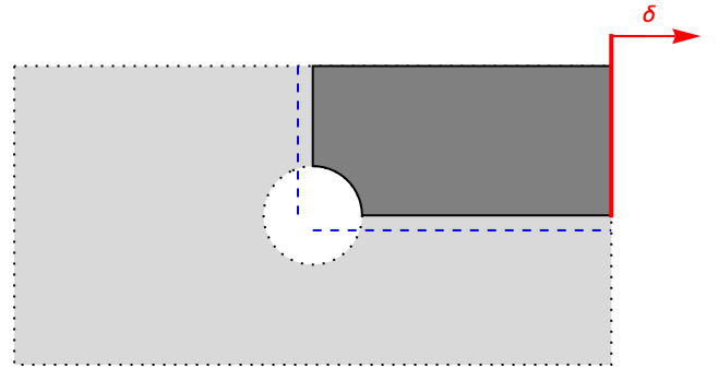
Holed plate geometry. Thanks to the symmetry, the problem is reduced to a quarter where the left and bottom sides, shown in dashed blue, can slide and a displacement is applied on the right side, marked in red.
Due to the symmetry of the plate, only one quarter is considered in this investigation. Symmetry conditions are applied along the left and bottom edges, while the right edge is subjected to displacement.
l = 0.04;
h = 0.02;
t = 0.001;reg = RegionDifference[Rectangle[{0, 0}, {l, h}], Disk[{0, 0}, h / 3]]mesh = ToElementMesh[reg, "MaxCellMeasure" -> 1.5 10^-6];vars = {{u[x, y], v[x, y], w[x, y]}, {x, y, z}};pars = <|"YoungModulus" -> 70 * 10^9, "PoissonRatio" -> 0.3, "Thickness" -> t, "SolidMechanicsModelForm" -> "ExtendedPlaneStrain"|>;δ = 1.5 * 10^-3;Γsym = {SolidDisplacementCondition[x == 0, vars, pars, <|"Displacement" -> {0, None}|>], SolidDisplacementCondition[y == 0, vars, pars, <|"Displacement" -> {None, 0}|>]};eqn[vars_, pars_, δ_] := {SolidMechanicsPDEComponent[vars, pars] == {0, 0}, Γsym, SolidDisplacementCondition[x == l, vars, pars, <|"Displacement" -> {δ, None}|>]}Initially, the mechanical problem is solved assuming fully elastic behavior. This solution serves as the starting point for the subsequent elasto-plastic computation.
elasticDispl = NDSolveValue[eqn[vars, pars, δ], vars[[1]], {x, y}∈mesh];strainE = SolidMechanicsStrain[vars, pars, elasticDispl];
stressE = SolidMechanicsStress[vars, pars, strainE];
vmE = Head@ VonMisesStress[vars, pars, stressE];parsPlastic = pars;
parsPlastic["YieldStress"] = 250 * 10^7;
parsPlastic["HardeningModulus"] = 150 * 10^8;RegionPlot[{vmE[x, y] >= parsPlastic["YieldStress"], vmE[x, y] < parsPlastic["YieldStress"]}, {x, y}∈mesh, ...]maxIteration = 100;
elastoplasticDispl = elasticDispl;
updatePars = PDEModels`InitializePlasticity[vars, parsPlastic, elastoplasticDispl];
Monitor[
i = 1;
While[PDEModels`PlasticStepQ[vars, updatePars] && i < maxIteration,
updatePars = PDEModels`PlasticStrainStep[vars, updatePars, elastoplasticDispl];
elastoplasticDispl = NDSolveValue[eqn[vars, updatePars, δ], vars[[1]], {x, y}∈mesh];
i++;],
i]Legended[Show[
mesh[...],
ElementMeshDeformation[mesh, elasticDispl[[1 ;; 2]], "ScalingFactor" -> 5][...],
ElementMeshDeformation[mesh, elastoplasticDispl[[1 ;; 2]], "ScalingFactor" -> 5][...]],
SwatchLegend[{LightGray, Blue, Red}, {"Undeformed", "Elastic", "Elastoplastic"}]]As can be observed, the holed geometry results in high deformation and stress concentrations near the upper boundary of the hole. Consequently, plastic strain localizes in this area, causing a slight change in the final deformation, particularly in the top-left area.
strainEP = SolidMechanicsStrain[vars, updatePars, elastoplasticDispl];
stressEP = SolidMechanicsStress[vars, updatePars, strainEP];
vmEP = Head@ VonMisesStress[vars, updatePars, stressEP];pt = {h / 2.9, h / 2.9};σVMEP = vmEP@@ptσVME = vmE@@ptIt is possible to visualize the stress state directly on the stress-strain curve.
ϵ0 = σy0 / Y;eCurve = ϵ * Y;
epCurve = {{0, 0}, {ϵ0, σy0}, {ϵf, σy0 + H * (ϵf - ϵ0)}};rep = {ϵf -> 0.065, σy0 -> parsPlastic["YieldStress"], Y -> parsPlastic["YoungModulus"], H -> parsPlastic["HardeningModulus"]};pointE = {σVME / Y, σVME} /. rep;
pointEP = {σVME / Y, σVMEP} /. rep;Show[
Plot[{σy0 /. rep, eCurve /. rep}, {ϵ, 0, ϵf /. rep}, ...],
ListLinePlot[epCurve /. rep, Rule[...]],
ListPlot[{{pointE}, {pointEP}}, ...]] /. repHere, the effect of the elasto-plastic model with linear hardening is observed. The stress values predicted by the fully elastic model, dashed orange, exceed the yielding threshold, dashed blue. When using the elasto-plastic model, the stress is instead limited to a new value defined along the hardening line, solid blue. Note that, unlike the perfect plasticity case, the final stress state is higher than the original yield limit.
Load History
In plasticity, the material response is path dependent, meaning that its behavior at any given moment depends not only on the current load but also on the entire load history. This dependence manifests in two key ways: through the accumulation of permanent deformation and through the way the material’s internal state evolves as a variable load drives the system along different segments of the yield surface, influencing the direction and magnitude of further plastic flow.
Permanent Deformation
An important characteristic of an elasto-plastic model is its ability to capture permanent plastic deformation. Once the material exceeds the yield point, plastic deformation begins, leading to a permanent change in shape that remains even after the load is removed.
In the following example, the 2D beam-like structure of the introductory example undergoes permanent deformation due to an imposed displacement that causes an excessive stress. After yielding, the structure is unloaded, and the final deformed configuration clearly exhibits residual deformation, indicating the permanent effects of plasticity.
mesh = ToElementMesh[Rectangle[{0, 0}, {10, 1}], "MeshElementType" -> TriangleElement, "MaxCellMeasure" -> 0.06];vars = {{u[x, y], v[x, y], 0}, {x, y, z}};pars = <|"YoungModulus" -> 90 * 10^9, "PoissonRatio" -> 0.3, "Thickness" -> 0.01, "SolidMechanicsModelForm" -> "ExtendedPlaneStrain"|>;parsPlastic = pars;
parsPlastic["YieldStress"] = 650 * 10^6;eqn[vars_, pars_, imposedDispl_] := {SolidMechanicsPDEComponent[vars, pars] == {0, 0}, SolidFixedCondition[x == 0, vars, pars],
SolidDisplacementCondition[x == 10, vars, pars, <|"Displacement" -> {None, imposedDispl}|>]}Initially, the mechanical problem is solved assuming fully elastic behavior. This solution serves as the starting point for the subsequent elasto-plastic computation.
δ = -1.15;elasticDispl = NDSolveValue[eqn[vars, pars, δ], vars[[1]], {x, y}∈mesh];strainE = SolidMechanicsStrain[vars, pars, elasticDispl];
stressE = SolidMechanicsStress[vars, pars, strainE];
vmE = Head@VonMisesStress[vars, pars, stressE]RegionPlot[{vmE[x, y] >= parsPlastic["YieldStress"], vmE[x, y] < parsPlastic["YieldStress"]}, {x, y}∈mesh, ...]Next, the elasto-plastic model is used to compute the results.
maxIteration = 100;
elastoplasticDispl = elasticDispl;
updatePars = PDEModels`InitializePlasticity[vars, parsPlastic, elastoplasticDispl];
Monitor[
	i = 1;
	While[PDEModels`PlasticStepQ[vars, updatePars] && i < maxIteration,
	updatePars = PDEModels`PlasticStrainStep[vars, updatePars, elastoplasticDispl];
	elastoplasticDispl = NDSolveValue[eqn[vars, updatePars, δ], vars[[1]], {x, y}∈mesh];
	i++;],
i]Finally, the solid constraint boundary conditions are removed, leaving the model with just fixed conditions. The solution is then recomputed. It is important to note that the resulting solution is nontrivial, as the updatedPars contains the information necessary to compute the deformation associated with the plastic strain.
noLoadDispl = NDSolveValue[eqn[vars, updatePars, None], vars[[1]], {x, y}∈mesh];scalingFactor = 2;elasticDeformedMesh = ElementMeshDeformation[mesh, elasticDispl[[1 ;; 2]], "ScalingFactor" -> scalingFactor];elastoplasticDeformedMesh = ElementMeshDeformation[mesh, elastoplasticDispl[[1 ;; 2]], "ScalingFactor" -> scalingFactor];plasticizedMesh = ElementMeshDeformation[mesh, noLoadDispl[[1 ;; 2]], "ScalingFactor" -> scalingFactor];As shown in the following figure, the final configuration shown in black exhibits a permanent plastic deformation. Note that the elasto-plastic and purely elastic responses appear quite similar, as both are driven by the same imposed displacement on the right side. However, the final plasticized configuration is slightly less deformed than the other ones, since the entire elastic contribution is recovered upon unloading.
Legended[Show[
mesh[...],
	elasticDeformedMesh[...],
elastoplasticDeformedMesh[...],
 plasticizedMesh[...]],
SwatchLegend[...]]
How can the effect of plastic deformation be visualized? The most relevant indicator of deformation due to plasticity is the plastic strain. To identify the regions that have undergone plastic deformation, one can examine the equivalent plastic strain, which provides a single positive scalar value representing a weighted average of the components of the plastic strain tensor.
plasticStrain = PDEModels`PlasticStrain[vars, updatePars]equivalentPlasticStrain = EquivalentStrain[vars, updatePars, plasticStrain];maxPS = Max[Head[equivalentPlasticStrain]["ValuesOnGrid"]]mappedEquivalentStrain = ElementMeshInterpolation[plasticizedMesh, Head[equivalentPlasticStrain]["ValuesOnGrid"]];Show[mesh["Wireframe"["MeshElement" -> "BoundaryElements", "MeshElementStyle" -> Gray]],
DensityPlot[mappedEquivalentStrain[x, y], {x, y}∈plasticizedMesh, ...]
]As shown in the plot, the curvature of the beam is primarily influenced by the large strain developed near the fixed end, where higher stress levels are reached during the loading phase.
The loading path refers to the trajectory in the stress–strain plane. Once the yield point is exceeded, the material begins to undergo plastic deformation, resulting in permanent strain. In the following analysis, the loading path is examined at a representative point located in the highly plasticized region, with coordinates (0.3, 0.98).
pt = {0.3, 0.98};strainEP = SolidMechanicsStrain[vars, updatePars, elastoplasticDispl];
stressEP = SolidMechanicsStress[vars, updatePars, strainEP];
vmEP = Head@ VonMisesStress[vars, updatePars, stressEP];σE = vmE@@ptσEP = vmEP@@ptϵtotal = σE / pars["YoungModulus"];In the above, the total strain was computed. Since there are no other strains involved, the total strain is also the elastic strain ![]() .
.
In the elasto-plastic model, the same displacement boundary condition is applied, so the total strain remains unchanged. However, since the elastic and plastic components contribute differently, the resulting stress state is not the same.
ϵyield = parsPlastic["YieldStress"] / pars["YoungModulus"];Since this is a perfect plasticity model, the stress obtained from the elasto-plastic solution remains constant and equal to the yield stress.
A small numerical discrepancy may appear when evaluating the stress at a specific point. This effect is due to result interpolation.
(parsPlastic["YieldStress"] - σEP/parsPlastic["YieldStress"])All these quantities can be visualized on the strain-stress plane.
p1 = {ϵyield, parsPlastic["YieldStress"]};p2 = {ϵtotal, σEP};line = y - p2[[2]] == pars["YoungModulus"] (x - p2[[1]]);
unloading = SolveValues[line, y][[1]]permanentStrain = SolveValues[unloading == 0, x][[1]]p3 = {permanentStrain, 0};Show[Plot[{σEP, ϵ * pars["YoungModulus"]}, {ϵ, 0, ϵf = 0.016}, ...],
ListLinePlot[{{0, 0}, {ϵyield, σEP}, {ϵf, σEP}}],
ListPlot[{{p1}, {p2}, {p3}}, ...],
Graphics[Arrow[{p2, {permanentStrain, 0}}]]
]One of the most important features of an elasto-plastic model is its capability to represent permanent deformation. In a purely elastic model, loading and unloading occur along the same path, a straight line defined by Young’s modulus as the slope. No permanent deformation occurs in this case.
When plastic behavior is introduced, however, the material begins to deform plastically once it exceeds the yield point P1. From this point, the stress-strain curve deviates from the elastic line. In the case of a perfect plastic law, the material behavior follows a horizontal path, with constant stress at the yield level, up to the imposed total strain in P2.
Upon unloading, the material recovers its elastic component: it unloads along a line with the same slope defined by Young’s modulus. However, after removing all external constraints, a residual, or permanent, deformation remains due to the plastic behavior. It is highlighted by the point P3.
Load History
In the next section, a prescribed displacement history is applied. Now each increment influences the subsequent response. A progressively increasing displacement is imposed and then followed by a progressive return to zero. This will result in two notable effects: the final deformation will remain nonzero, and the stress–strain response will trace a characteristic elasto-plastic hysteresis loop.
The previously introduced holed plate is taken as the numerical example. The displacement imposed as a boundary condition, which was previously applied with the value ![]() , is now scaled by a multiplier that varies at each load step and defines the load history.
, is now scaled by a multiplier that varies at each load step and defines the load history.
δmax = 3.9 10^-3;multipliers = Table[1 - Abs[(k - 1)], {k, 0.1, 2 , 1 / 10}];The applied displacement is gradually increased up to ![]() and then reduced back to zero. A list of multipliers, ranging between 0 and 1, is used to scale the maximum displacement and define each load step. Ten steps are employed to reach the maximum displacement, followed by another 10 steps to gradually return to zero. This sequence defines the load history.
and then reduced back to zero. A list of multipliers, ranging between 0 and 1, is used to scale the maximum displacement and define each load step. Ten steps are employed to reach the maximum displacement, followed by another 10 steps to gradually return to zero. This sequence defines the load history.
It is important that each step be sufficiently small to ensure an accurate capture of the yield point. In addition, using smaller steps improves convergence, as the elasto-plastic solution at each load step remains close to the one of the previous step.
ListLinePlot[multipliers, ...]To follow the load history, the elasto-plastic problem is solved incrementally at each step. At every step, the plastic solution from the previous step serves as the starting point, ensuring that the final result reflects the entire history of plastic evolution.
l = 0.04;
h = 0.02;
t = 0.001;reg = RegionDifference[Rectangle[{0, 0}, {l, h}], Disk[{0, 0}, h / 3]]mesh = ToElementMesh[reg, "MaxCellMeasure" -> 1.5 10^-6];vars = {{u[x, y], v[x, y], w[x, y]}, {x, y, z}};pars = <|"YoungModulus" -> 70 * 10^9, "PoissonRatio" -> 0.3, "Thickness" -> t, "SolidMechanicsModelForm" -> "ExtendedPlaneStrain"|>;parsPlastic = pars;
parsPlastic["YieldStress"] = 250 * 10^7;
parsPlastic["HardeningModulus"] = 150 * 10^8;Γsym = {SolidDisplacementCondition[x == 0, vars, pars, <|"Displacement" -> {0, None}|>], SolidDisplacementCondition[y == 0, vars, pars, <|"Displacement" -> {None, 0}|>]};eqn[vars_, pars_, δ_] := {SolidMechanicsPDEComponent[vars, pars] == {0, 0}, Γsym, SolidDisplacementCondition[x == l, vars, pars, <|"Displacement" -> {δ, None}|>]}Each step is treated as a separate elasto-plastic problem. The solution begins with an elastic trial state, which is then corrected through an elasto-plastic iteration if the stress exceeds the yield limit. The initialization of each step takes into account the updated material state from the preceding step, ensuring continuity of the plastic evolution.
loadStepElastoPlastic[{previousPars_, _}, δ_] := Module[{updatePars, elastoplasticDispl},
	updatePars = PDEModels`PlasticityHistory[vars, previousPars];
	elastoplasticDispl = NDSolveValue[eqn[vars, updatePars, δ], vars[[1]], {x, y}∈mesh];
	updatePars = PDEModels`InitializePlasticity[vars, updatePars, elastoplasticDispl];
	i = 1;
	While[PDEModels`PlasticStepQ[vars, updatePars] && i < maxIteration,
	updatePars = PDEModels`PlasticStrainStep[vars, updatePars, elastoplasticDispl];
	elastoplasticDispl = NDSolveValue[eqn[vars, updatePars, δ], vars[[1]], {x, y}∈mesh];
	i++;];
	{updatePars, elastoplasticDispl}
]maxIteration = 150;elasticDispl = NDSolveValue[eqn[vars, pars, multipliers[[1]] * δmax ], vars[[1]], {x, y}∈mesh];result = {parsPlastic, elasticDispl};
Monitor[AbsoluteTiming[
results = Table[result = loadStepElastoPlastic[result, m * δmax]
, {m, multipliers}];], m]meshes = ElementMeshDeformation[mesh, #[[1 ;; 2]], "ScalingFactor" -> 3]& /@ results[[All, 2]];imgs = MapThread[Function[{multiplier, meshElement},
GraphicsColumn[ {Text["Applied displacement: " <> ToString[NumberForm[multiplier, {∞, 2}]] <> " δ"],
Show[mesh["Edgeframe"], meshElement["Wireframe"["MeshElementStyle" -> EdgeForm[Blue]]], PlotRange -> {{0., 0.052}, {0., 0.02}}]}, ImageSize -> Medium]],
{multipliers, meshes} ];
ListAnimate[imgs]pt = {Cos[π / 4], Sin[π / 4]}h / 2.1At each step, the applied displacement is increased, and the material response follows the hardening model, leading to a progressive accumulation of plastic strain. After the maximum displacement is reached, plastic strain remains even as the displacement decreases. This results in a gradual compression of the material. To observe this effect, one can examine the stress and strain along the displacement direction.
evaluateQuantities[{pars_, displ_}] := Module[{strain, stress},
	strain = SolidMechanicsStrain[vars, pars, displ];
	stress = SolidMechanicsStress[vars, pars, strain];
	{Head[strain[[1, 1]]][pt[[1]], pt[[2]]],
	Head[stress[[1, 1]]][pt[[1]], pt[[2]]]}
]values = Table[evaluateQuantities[r], {r, results}];Show[
ListPlot[values[[{11}]], ...],
ListLinePlot[values, ...] ,
ListPlot[values[[{4}]], ...],
ListPlot[values[[{-4}]], ...]
]As mentioned before, yielding becomes clearly evident after the fourth loading step, with the stress–strain response following the hardening line. Notably, after reaching the maximum applied displacement ![]() , the subsequent progressive reduction in the imposed displacement results in a new compressive state at the point of interest. Note that this effect can only be observed using a stress measure that preserves the sign, and it cannot be detected by considering only the von Mises stress.
, the subsequent progressive reduction in the imposed displacement results in a new compressive state at the point of interest. Note that this effect can only be observed using a stress measure that preserves the sign, and it cannot be detected by considering only the von Mises stress.
generatePlotImg[j_] := Module[{img, strain, stress, interp},
	strain = SolidMechanicsStrain[vars, results[[j, 1]], results[[j, 2]]];
	stress = SolidMechanicsStress[vars, results[[j, 1]], strain];
	interp = ElementMeshInterpolation[meshes[[j]], Head[stress[[1, 1]]]["ValuesOnGrid"]];
	img  = Show[
	mesh[...], DensityPlot[interp[x, y], {x, y}∈meshes[[j]], ...], ...];
	img
]plots = Table[generatePlotImg[j], {j, Length[multipliers]}];ListAnimate[plots]Because the displacement is applied uniaxially, the final displacement on the right side is zero, while the top edge shows deformation as a result of material plasticization.
It is important to note that a zero-stress state does not exist. Even in the final step, where the overall displacement returns to zero, the stress state indicates compression. This occurs because plastic strain has accumulated, modifying the material’s stress response in accordance with the hardening law.
References
1. Lubliner, J. Plasticity Theory. Dover, 2008. ISBN 978-0-486-46290-5.
2. Wrigger, P. Nonlinear Finite Element Methods. Springer, 2008. ISBN 978-3-540-71001-1.