

AsymptoticOutputTracker
AsymptoticOutputTracker[sys,{f1,…},{p1,…}]
gives the state feedback control law that causes the outputs of the affine system sys to track the reference signals fi with decay rates pj.
AsymptoticOutputTracker[{sys,{out1,…},{in1,…}},…]
specifies outputs outi and control inputs inj to use.
Details and Options
- The system sys can be a StateSpaceModel or AffineStateSpaceModel.
- The reference signals fi should be pure functions of a single variable.
- The decay rates pi correspond to pole locations for the closed-loop system, and the number of poles pi is given by Total[SystemsModelVectorRelativeOrders[sys]].
- The outputs {out1,…} and inputs {in1,…} are part specifications and by default are taken to be All.
- The number of outputs and reference signals must be the same.
- AsymptoticOutputTracker is based on FeedbackLinearize, and any residual dynamics must be stable for valid results. »

Examples
open all close allBasic Examples (1)
A linear single-output system tracking a sinusoid:
ssm = StateSpaceModel[{{{-3}}, {{1}}, {{1}}, {{0}}}, {{x[t], 2}}, Automatic,
 Automatic, t, SamplingPeriod -> None, SystemsModelLabels -> None];
ref = Sin[t];fb = AsymptoticOutputTracker[ssm, ref, {-5}]csys = SystemsModelStateFeedbackConnect[ssm, fb]After initial transients, the output tracks the reference:
y = OutputResponse[csys, {0}, {t, 0, 8}];Plot[{y, ref}, {t, 0, 8}, PlotLegends -> {"output", "reference"}]Scope (4)
An affine system tracking a piecewise constant signal:
assm = AffineStateSpaceModel[{{Subscript[x, 2], Subscript[x, 1] +
    Subscript[x, 2]}, {{0}, {1 + Subscript[x, 1]}},
  {Subscript[x, 1]}, {{0}}}, {{Subscript[x, 1], 1},
  {Subscript[x, 2], 0}}, Automatic, {Automatic}, t,
SamplingPeriod -> None];ref = Piecewise[{{1, 0 ≤ t ≤ 5}, {2, 5 < t ≤ 10}, {1, 10 < t ≤ 15}}, 0];Plot[ref, {t, 0, 20}, PlotStyle -> Thick]fb = AsymptoticOutputTracker[assm, ref, {-3, -4}]Simulate the closed-loop system:
csys = SystemsModelStateFeedbackConnect[assm, fb];
y = OutputResponse[csys /. Indeterminate -> 0, {0}, {t, 0, 20}];Plot[y, {t, 0, 20}, PlotRange -> All, AxesOrigin -> {0, 0}]Generate a trajectory passing through random points:
pts = Thread[{Range[0, 50, 5], RandomReal[{-10, 10}, 11]}];ref = Interpolation@pts;
Plot[ref[t], {t, 0, 50}]Design a feedback law that causes an affine system to track the trajectory:
assm = AffineStateSpaceModel[{{Subscript[x, 1] + Subscript[x, 2],
   Subscript[x, 1] - 2*Subscript[x, 2] -
    Subscript[x, 1]*Subscript[x, 3],
   Subscript[x, 1] + Subscript[x, 1]*Subscript[x, 2] -
    4*Subscript[x, 3]}, {{0}, {1}, {0}}, {Subscript[x, 1]}, {{0}}},
 {Subscript[x, 1], Subscript[x, 2], Subscript[x, 3]},
Automatic, {Automatic}, t, SamplingPeriod -> None];fb = AsymptoticOutputTracker[assm, ref[t], {-4 + I, -4 - I}];Simulate the closed-loop system:
csys = SystemsModelStateFeedbackConnect[assm, fb];
y = OutputResponse[csys, {0}, {t, 0, 50}];Plot[y, {t, 0, 50}, Epilog -> {PointSize[Medium], Point[pts]}]If there are more inputs than outputs, some of the feedback inputs are zero:
ssm = StateSpaceModel[{{{-1, 0}, {0, -2}}, {{1, 2}, {1, -1}}, {{1, 2}}, {{0, 0}}},
 {{Subscript[x, 1][t], -1},
  {Subscript[x, 2][t], 1}},
 {Subscript[u, 1][t], Subscript[u, 2][t]},
 Automatic, t, SamplingPeriod -> None, SystemsModelLabels -> None];
ref = Sin[t];fb1 = AsymptoticOutputTracker[ssm, ref, {-5, -8}]Specify the second input to use for control feedback:
fb2 = AsymptoticOutputTracker[{ssm, All, 2}, ref, {-5, -8}]Compute the closed-loop systems in each case:
csys1 = SystemsModelStateFeedbackConnect[ssm, fb1]csys2 = SystemsModelStateFeedbackConnect[ssm, fb2, All, {2}]Both the controllers achieve tracking:
y1 = OutputResponse[csys1, {0}, {t, 0, 12}];
y2 = OutputResponse[csys2, {0}, {t, 0, 12}];Plot[{y1, y2}, {t, 0, 12}]Specify the outputs to track and control inputs to use:
ssm = StateSpaceModel[{{{0, 1, 0, 0}, {-2, -3, 0, 0}, {0, 0, 0, 1}, {0, 0, -2, -3}},
  {{0, 0}, {1, 0}, {0, 0}, {0, 1}}, {{2, 1, 2, 2}, {1, 1, 2, 1}}, {{0, 0}, {0, 0}}}];
outs = {1};
inps = {2};
Design a feedback control law:
ref = Sin[t];
fb = AsymptoticOutputTracker[{ssm, {1}, {2}}, ref, {-10, -11}]csys = SystemsModelStateFeedbackConnect[ssm, fb, All, {2}]The response of the first output:
or = OutputResponse[csys, {0, 0}, {t, 0, 10}][[1]]Plot[{or, ref}, {t, 0, 10}]Applications (3)
Design a controller for a flexible joint to track a specified trajectory while carrying a load at one end: »
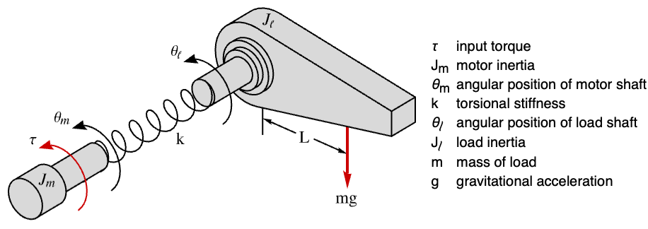
pars = {Subscript[J, m] -> 0.4, k -> 100, Subscript[J, l] -> 1, M -> 1.5, g -> 9.8, L -> 0.4};assm = AffineStateSpaceModel[{Subscript[J, l] Subscript[θ, l]''[t] + M g L Sin[Subscript[θ, l][t]] + k(Subscript[θ, l][t] - Subscript[θ, m][t]) == 0, Subscript[J, m] Subscript[θ, m]''[t] - k(Subscript[θ, l][t] - Subscript[θ, m][t]) == τ[t]}, {Subscript[θ, l][t], Subscript[θ, l]'[t], Subscript[θ, m][t], Subscript[θ, m]'[t]}, τ[t], {Subscript[θ, l][t]}, t]The joint needs to be rotated from 5° to ![]() in 10 seconds:
in 10 seconds:
traj = 5 ° + -3 ° t^2 / 5 + 1° t^3 / 25;
Plot[traj, {t, 0, 10}]
The trajectory starts and ends with zero velocity and is smooth:
{Plot[Evaluate@D[traj, t], {t, 0, 10}], Plot[Evaluate@D[traj, {t, 2}], {t, 0, 10}]}Obtain a computed torque control law:
cinps = AsymptoticOutputTracker[assm, #, {-7 + 2I, -7 - 2 I, -9, -10}]& /@ {traj, -15 °}//Flatten;csys = SystemsModelStateFeedbackConnect[assm, {Piecewise[{{cinps[[1]], 0 ≤ t ≤ 10}}, cinps[[2]]]}];The joint follows the trajectory after initial transients and remains at ![]() after 10 seconds:
after 10 seconds:
OutputResponse[{csys /. pars, {5 °, 0, 0, 0}}, {0}, {t, 0, 15}];Plot[Evaluate@{traj, %}, {t, 0, 15}]Compute a control law for a stepper motor to position a load at 1° in 0.1 seconds along the trajectory of a first-order system. A model of the motor: »
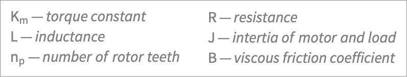
pars = {Subscript[K, m] -> 2 / 10, R -> 45 / 100, L -> 2 / 1000, J -> 65 / 10000, Subscript[n, p] -> 30, B -> 10 / 10000};asys = AffineStateSpaceModel[
{{(Sin[Subscript[n, p]*θ[t]]*
Subscript[K, m]*Subscript[n, p]*
ω[t] - R*Subscript[i, a][
t])/L,
((-Cos[Subscript[n, p]*θ[t]])*
Subscript[K, m]*Subscript[n, p]*
ω[t] - R*Subscript[i, b][
t])/L, ω[t],
((-B)*ω[t] +
Cos[Subscript[n, p]*θ[t]]*
Subscript[K, m]*Subscript[n, p]*
Subscript[i, a][t] -
Sin[Subscript[n, p]*θ[t]]*
Subscript[K, m]*Subscript[n, p]*
Subscript[i, b][t])/J},
{{L^(-1), 0}, {0, L^(-1)}, {0, 0}, {0, 0}},
{θ[t]}, {{0, 0}}},
{{Subscript[i, a][t], 0},
{Subscript[i, b][t], 0},
{θ[t], 0}, {ω[t], 0}},
{{vsa[t], 0}, {vsb[t], 0}}, {Automatic},
t, SamplingPeriod -> None] /. pars;ref = OutputResponse[TransferFunctionModel[{{{1}}, 1 + s/100}, s], UnitStep[t], {t, 0, 0.1}];
Plot[ref, {t, 0, 0.1}, PlotRange -> All]Short[fb = AsymptoticOutputTracker[asys, ref, {-300, -500, -600}]]The closed-loop system has the desired response:
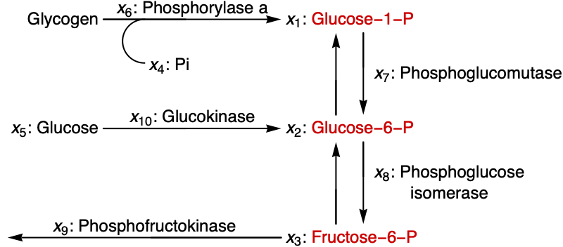
SystemsModelStateFeedbackConnect[asys, fb];Plot[Evaluate@OutputResponse[%, {0, 0}, {t, 0, 0.1}], {t, 0, 0.1}, PlotRange -> All]The glycolytic-glycogenolytic pathway, where the rates of metabolites ![]() ,
, ![]() , and
, and ![]() are taken as the manipulated variables, and
are taken as the manipulated variables, and ![]() ,
, ![]() ,
, ![]() , and
, and ![]() are kept constant. Design a feedback law that maintains the values of the metabolites
are kept constant. Design a feedback law that maintains the values of the metabolites ![]() ,
, ![]() , and
, and ![]() at 0.2, 0.5, and 0.4: »
at 0.2, 0.5, and 0.4: »
constants = {Subscript[x, 6][t] -> 3, Subscript[x, 7][t] -> 40, Subscript[x, 9][t] -> 2.86, Subscript[x, 10][t] -> 4};asys = AffineStateSpaceModel[
{{0.07788*Subscript[x, 4][t]^0.66*Subscript[x, 6][
t] - (1.0627*Subscript[x, 1][t]^1.53*
Subscript[x, 7][t])/Subscript[x, 2][t]^
0.59, (-0.00079*Subscript[x, 2][t]^3.97*
Subscript[x, 8][t])/Subscript[x, 3][t]^
3.06 + (0.585*Subscript[x, 1][t]^0.95*
Subscript[x, 5][t]^0.32*
Subscript[x, 7][t]^0.62*
Subscript[x, 10][t]^0.38)/
Subscript[x, 2][t]^0.41,
(0.00079*Subscript[x, 2][t]^3.97*Subscript[x, 8][
t])/Subscript[x, 3][t]^3.06 -
1.0588*Subscript[x, 3][t]^0.3*Subscript[x, 9][
t], 0, 0, 0}, {{0, 0, 0}, {0, 0, 0}, {0, 0, 0}, {1, 0, 0}, {0, 1, 0},
{0, 0, 1}}, {Subscript[x, 1][t],
Subscript[x, 2][t], Subscript[x, 3][t]},
{{0, 0, 0}, {0, 0, 0}, {0, 0, 0}}}, {{Subscript[x, 1][t], 0.067},
{Subscript[x, 2][t], 0.465},
{Subscript[x, 3][t], 0.15},
{Subscript[x, 4][t], 10},
{Subscript[x, 5][t], 5}, {Subscript[x, 8][t],
136}}, Automatic, {Automatic, Automatic, Automatic}, t, SamplingPeriod -> None] /. constants;A feedback law that maintains the values of ![]() ,
, ![]() , and
, and ![]() at 0.2, 0.5, and 0.4:
at 0.2, 0.5, and 0.4:
fb = AsymptoticOutputTracker[asys, {0.2, 0.5, 0.4}, {-0.5 + I, -0.5 - I, -1 + I , -1 - I, -2, -2.5}];Simulate the closed-loop system:
csys = SystemsModelStateFeedbackConnect[asys, fb];
Plot[Evaluate@OutputResponse[csys, {0, 0, 0}, {t, 0, 7}], {t, 0, 7}]fb /. Thread[{Subscript[x, 1][t], Subscript[x, 2][t], Subscript[x, 3][t], Subscript[x, 4][t], Subscript[x, 5][t], Subscript[x, 8][t]} -> StateResponse[csys, {0, 0, 0}, {t, 0, 7}]];GraphicsRow[Table[Plot[i, {t, 0, 7}, PlotRange -> All, ImageSize -> 145], {i, %}]]Properties & Relations (2)
The number of decay rates to be specified is determined by the sum of the vector relative orders:
assm = AffineStateSpaceModel[{{-Subscript[x, 1][t],
   -Subscript[x, 2][t] + Subscript[x, 2][t]^2,
   0}, {{1 + Subscript[x, 1][t]}, {1}, {1}},
  {Subscript[x, 3][t]}, {{0}}},
 {Subscript[x, 1][t], Subscript[x, 2][t],
  Subscript[x, 3][t]}, {u[t]}, {Automatic},
 t, SamplingPeriod -> None];
This indicates that a single decay rate needs to be specified:
Total@SystemsModelVectorRelativeOrders[assm]AsymptoticOutputTracker[assm, Sin[t], {-2}]The decay rates for each output are assigned based on its relative order:
assm = AffineStateSpaceModel[{{Subscript[x, 2][t] +
Subscript[x, 2][t]^2, Subscript[x, 3][t] -
Subscript[x, 1][t]*Subscript[x, 4][t] +
Subscript[x, 4][t]*Subscript[x, 5][t],
Subscript[x, 2][t]*Subscript[x, 4][t] +
Subscript[x, 1][t]*Subscript[x, 5][t] -
Subscript[x, 5][t]^2, Subscript[x, 5][t],
Subscript[x, 2][t]^2},
{{0, 1}, {0, 0}, {Cos[Subscript[x, 1][t] -
Subscript[x, 5][t]], 1}, {0, 0}, {0, 1}},
{Subscript[x, 1][t] - Subscript[x, 5][t],
Subscript[x, 4][t]}, {{0, 0}, {0, 0}}},
{{Subscript[x, 1][t], 0.1},
{Subscript[x, 2][t], 0.3},
{Subscript[x, 3][t], 0}, {Subscript[x, 4][t],
0.4}, {Subscript[x, 5][t], 1}},
{Subscript[, 1][t], Subscript[, 2][t]}, {Automatic, Automatic},
t, SamplingPeriod -> None];There are three decay rates needed for output 1 and two decay rates for output 2:
SystemsModelVectorRelativeOrders[assm]Specify slow rates ![]() for output 1 and fast rates
for output 1 and fast rates ![]() for output 2:
for output 2:
ref = {Sin[t], Cos[t]};
fb = AsymptoticOutputTracker[assm, ref, {-2, -3, -4, -10, -12}]
Output 2 will track faster than output 1:
or = OutputResponse[SystemsModelStateFeedbackConnect[assm, fb], {0, 0}, {t, 0, 3}];Plot[{or, ref}, {t, 0, 3}, PlotLegends -> {"output 1", "output 2", "ref 1", "ref 2"}]Possible Issues (1)
For the feedback law to be effective, any residual dynamics must be stable:
asys = AffineStateSpaceModel[{{Subscript[x, 1] - Subscript[x, 2],
   Subscript[x, 1] - Subscript[x, 2],
   3*Subscript[x, 2] + Subscript[x, 3] +
    (Subscript[x, 1] + Subscript[x, 2] + Subscript[x, 3])^
     2}, {{0}, {-1 - Subscript[x, 1]*Subscript[x, 2]},
   {1 + Subscript[x, 1]*Subscript[x, 2]}},
  {Subscript[x, 1]}, {{0}}}, {Subscript[x, 1],
  Subscript[x, 2], Subscript[x, 3]}, {v}, {Automatic},
Automatic, SamplingPeriod -> None];fb = AsymptoticOutputTracker[asys, 0.1, {-1.5, -0.5}]The feedback law is not effective:
SystemsModelStateFeedbackConnect[asys, fb];StateResponse[%, 0, {t, 0, 15}];This is because the residual dynamics are unstable:
FeedbackLinearize[asys, Automatic, "ResidualSystem"];Eigenvalues@First@Normal@StateSpaceModel@%Text
Wolfram Research (2014), AsymptoticOutputTracker, Wolfram Language function, https://reference.wolfram.com/language/ref/AsymptoticOutputTracker.html.
CMS
Wolfram Language. 2014. "AsymptoticOutputTracker." Wolfram Language & System Documentation Center. Wolfram Research. https://reference.wolfram.com/language/ref/AsymptoticOutputTracker.html.
APA
Wolfram Language. (2014). AsymptoticOutputTracker. Wolfram Language & System Documentation Center. Retrieved from https://reference.wolfram.com/language/ref/AsymptoticOutputTracker.html