

FullInformationOutputRegulator
FullInformationOutputRegulator[sys,rspec]
gives the full state information output regulator for sys using specification rspec.
FullInformationOutputRegulator[{sys,{out1,…},{in1,…}},…]
specifies the regulated outputs outi and the controlled inputs inj.
Details and Options
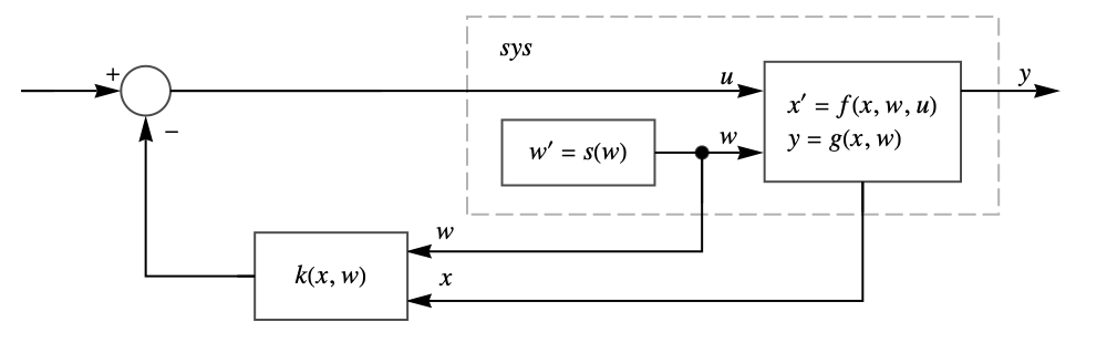
- FullInformationOutputRegulator returns a regulator that drives the sys outputs to zero and is typically used to suppress or track known inputs to the system.
- The system sys is taken to have state equations
 and
and  and outputs
  , with
  being the controllable input. The state
  is not affected by the input
  and is used to model signals to suppress or track, as indicated by the output function
  .
. - Typical output functions
 , which the regulator will drive to zero:
 -

suppress the effects of  on the states

cause  to track
- The system sys can be StateSpaceModel, AffineStateSpaceModel, or NonlinearStateSpaceModel.
- The computed state feedback
 regulates sys about an operating point using
  .
. - The state feedback
 has the form
  , where
  ,
,  , and
, and  is computed following rspec.
 - Possible regulator specifications rspec:
-
{"Poles",{p1,…}} computed with StateFeedbackGains {"Weights",{p,…}} computed with LQRegulatorGains {"Gains",κ} explicitly given gains - With the specification {"method",pars,opts}, the options opts are passed to the gain computation function.
- The outputs {out1,…} and inputs {in1,…} are part specifications and by default are taken to be All.
Examples
open all close allBasic Examples (1)
Compute the regulating feedback for a system with a constant disturbance of 0.5:
sys = AffineStateSpaceModel[{{w + 2*Subscript[x, 1] +
Subscript[x, 2], Subscript[x, 1] - 2*Subscript[x, 2],
0}, {{1}, {0}, {0}}, {Subscript[x, 1] + Subscript[x, 2]}, {{0}}},
{{Subscript[x, 1], 0}, {Subscript[x, 2], 0}, {w, 0.5}},
{Subscript[, 1]}, {Automatic}, Automatic, SamplingPeriod -> None];The regulator is a function of the states ![]() and the disturbance state
and the disturbance state ![]() :
:
k = FullInformationOutputRegulator[sys, {"Poles", {-1, -2}}]csys = SystemsModelStateFeedbackConnect[sys, k]The output is regulated to zero:
res1 = OutputResponse[{sys, {1, 1, 0.5}}, 0, {t, 0, 5}];
res2 = OutputResponse[{csys, {1, 1, 0.5}}, 0, {t, 0, 5}];Plot[{res1, res2}, {t, 0, 5}, PlotRange -> {0, 5}, PlotLegends -> {"unregulated", "regulated"}]Scope (8)
The regulator for a linear system with the exosystem pole at the origin:
FullInformationOutputRegulator[ssm = StateSpaceModel[{{{p, r}, {0, 0}}, {{b}, {0}},
{{c, 0}}, {{0}}}, SamplingPeriod -> None, SystemsModelLabels -> None], {"Poles", {Subscript[p, f]}}]SystemsModelStateFeedbackConnect[ssm, %]//SimplifyThe exosystem has a pair of complex poles:
ssm = StateSpaceModel[{{{p, Subscript[r, 1], Subscript[r, 2]},
   {0, 0, ω}, {0, -ω, 0}}, {{b}, {0}, {0}},
{{c, 0, 0}}, {{0}}}, SamplingPeriod -> None, SystemsModelLabels -> None];Assuming[ω ∈ Reals, FullInformationOutputRegulator[ssm, {"Poles", {Subscript[p, f]}}]]SystemsModelStateFeedbackConnect[ssm, %]//SimplifyThe exosystem's states are part of the regulator:
ssm = StateSpaceModel[{{{p, Subscript[r, 1], Subscript[r, 2]},
   {0, 0, ω}, {0, -ω, 0}}, {{b}, {0}, {0}},
  {{c, Subscript[c, 1], Subscript[c, 2]}}, {{0}}},
SamplingPeriod -> None, SystemsModelLabels -> None];Assuming[ω ∈ Reals, FullInformationOutputRegulator[ssm, {"Poles", {Subscript[p, f]}}]]SystemsModelStateFeedbackConnect[ssm, %]OutputResponse[{%, {Subscript[x, 10], Subscript[w, 10], Subscript[w, 20]}}, 0, t]//FullSimplifyThe system is regulated if pf is negative:
% /. Subscript[p, f] -> -5 /. Thread[{c, Subscript[c, 1], Subscript[c, 2], Subscript[x, 10], Subscript[w, 10], Subscript[w, 20]} -> RandomReal[1, 6]]Regulate an AffineStateSpaceModel:
Assuming[ω∈Reals, FullInformationOutputRegulator[AffineStateSpaceModel[{{p*x + x^2 +
Subscript[c, 1]*Subscript[w, 1] + Subscript[c, 2]*
Subscript[w, 2], ω*Subscript[w, 2],
(-ω)*Subscript[w, 1]}, {{b}, {0}, {0}},
{x}, {{0}}}, {x, Subscript[w, 1],
Subscript[w, 2]}, {Subscript[, 1]}, {Automatic}, Automatic,
SamplingPeriod -> None], {"Poles", {Subscript[p, f]}}]]Regulate a NonlinearStateSpaceModel:
FullInformationOutputRegulator[NonlinearStateSpaceModel[
 {{p*x + w*Subscript[c, 1] +
    u*Subscript[c, 2] + u*w*x*
     Subscript[c, 3], 0}, {x}}, {x, w},
 {u}, {Automatic}, Automatic, SamplingPeriod -> None], {"Poles", {Subscript[p, f]}}]
Specify the regulated outputs and feedback inputs:
FullInformationOutputRegulator[{StateSpaceModel[{{{0, 0}, {r, p}}, {{0, Subscript[b, 1]},
   {Subscript[b, 2], 0}}, {{1, 0}, {0, 1}}, {{0, 0}, {0, 0}}}, SamplingPeriod -> None,
 SystemsModelLabels -> None], {2}, {1}}, {"Poles", {Subscript[p, f]}}]
Use LQRegulatorGains to compute the stabilizing gains by specifying the weights:
FullInformationOutputRegulator[AffineStateSpaceModel[{{w + x, 0}, {{1}, {0}}, {x}, {{0}}},
{x, w}, {Subscript[, 1]}, {Automatic}, Automatic,
SamplingPeriod -> None], {"Weights", {{{1}}, {{1}}}}]FullInformationOutputRegulator[AffineStateSpaceModel[{{w + x, 0}, {{1}, {0}}, {x}, {{0}}},
{x, w}, {Subscript[, 1]}, {Automatic}, Automatic,
SamplingPeriod -> None], {"Gains", {{k}}}]Applications (6)
Reject a disturbance modeled as ![]() :
:
dModel = NonlinearStateSpaceModel[w''[t] + w[t] == 0, {{w[t], 0}, {w'[t], 1}}, {}, {}, t];The full model of the system with disturbance:
nsys = NonlinearStateSpaceModel[{{x[t] + Subscript[, 1][t] + v[t]}, {x[t]}}, {{x[t], 0}}, {v[t]}, Automatic, t];sys = SystemsModelMerge[{dModel, nsys}]k = FullInformationOutputRegulator[sys, {"Poles", {-2}}]csys = SystemsModelStateFeedbackConnect[sys, k]The output is regulated in the presence of the disturbance:
OutputResponse[{csys, {0, 1, 1}}, 0, {t, 0, 3}];Plot[%, {t, 0, 3}, PlotRange -> All]iModel = NonlinearStateSpaceModel[w''[t] + w[t] == 0, {{w[t], 0}, {w'[t], 1}}, {}, {}, t];The full model of the system and input model:
nsys = NonlinearStateSpaceModel[{{x[t] + Subscript[, 1][t] + v[t]}, {x[t], x[t] - Subscript[, 1][t]}}, {{x[t], 0}}, {Subscript[, 1][t], v[t]}, Automatic, t];sys = SystemsModelMerge[{iModel, nsys}]k = FullInformationOutputRegulator[{sys, 2}, {"Poles", {-2}}]csys = SystemsModelExtract[SystemsModelStateFeedbackConnect[sys, k], All, 1]or = OutputResponse[{csys, {0, 1, 0.5}}, 0, {t, 0, 10}];
Plot[or, {t, 0, 10}, PlotRange -> All]Simultaneously track a step input and reject a sinusoidal disturbance:
iModel = NonlinearStateSpaceModel[{{0}, {x - r}}, {{r, 1}}, {}]dModel = NonlinearStateSpaceModel[{{Subscript[w, 2], -Subscript[w, 1]}, {}}, {{Subscript[w, 1], 0}, {Subscript[w, 2], 1}}, {}]nsys = NonlinearStateSpaceModel[{{x + r + Subscript[w, 1] + v}, {x}}, {{x, 0}}, {r, Subscript[w, 1], v}]sys = SystemsModelMerge[{nsys, iModel, dModel}]k = FullInformationOutputRegulator[{sys, 2}, {"Poles", {-8}}]csys = SystemsModelExtract[SystemsModelStateFeedbackConnect[sys, k], All, 1]The simulation shows the output tracking a step signal:
OutputResponse[NonlinearStateSpaceModel[csys, {x -> -1, r -> 1, Subscript[w, 1] -> 0, Subscript[w, 2] -> 1}], 0, {t, 0, 5}];
Plot[%, {t, 0, 5}, PlotRange -> All]
Regulate an aircraft's longitudinal dynamics in the presence of disturbances:»
aircraft = StateSpaceModel[{{{0, 14.3877, 0, -31.5311}, {-0.0012, -0.4217, 1, -0.0284},
   {0.0002, -0.3816, -0.4658, 0}, {0, 0, 1, 0}}, {{0.7898, -0.6526, -0.335, 0.4637, 0.9185},
   {-0.00588, 0.0049, 0.0025, -0.0035, -0.0068}, {-0.2541, 0.21, 0.1078, -0.1492, -0.2959},
   {0, 0, 0, 0, 0}}, {{1, 0, 0, 0}}, {{0, 0, 0, 0, 0}}}, {Subscript[x, 1],
  Subscript[x, 2], Subscript[x, 3], Subscript[x, 4]},
 {u, Subscript[w, 1], Subscript[w, 2],
  Subscript[w, 3], Subscript[w, 4]}, SamplingPeriod -> None,
 SystemsModelLabels -> None];
The disturbances consist of two frequency components:
dist = StateSpaceModel[{{{0, -0.1, 0, 0}, {0.1, 0, 0, 0}, {0, 0, 0, -0.2}, {0, 0, 0.2, 0}},
  {{}, {}, {}, {}}, {}}, {Subscript[w, 1], Subscript[w, 2],
  Subscript[w, 3], Subscript[w, 4]}, SamplingPeriod -> None,
SystemsModelLabels -> None];sys = SystemsModelMerge[{aircraft, dist}]A control law that regulates the output (speed) in the presence of the disturbances:
fb = FullInformationOutputRegulator[sys, {"Poles", {-1, -2, -2.5 + I, -2.5 - I}}]csys = SystemsModelStateFeedbackConnect[sys, fb]Simulation showing regulation being achieved:
OutputResponse[{csys, {0.1, 0.001, 0, 0, 1, 0, 1, 0}}, 0, {t, 0, 8}];
Plot[%, {t, 0, 8}, PlotRange -> All]fb.StateResponse[{csys, {0.1, 0.001, 0, 0, 1, 0, 1, 0}}, 0, {t, 0, 150}];
Plot[%, {t, 0, 150}, PlotRange -> All]Regulate a Rössler prototype-4 system:»
asys = AffineStateSpaceModel[{{-Subscript[x, 2] - Subscript[x, 3],
   Subscript[x, 1],
   0.5*(Subscript[x, 2] - Subscript[x, 2]^2) -
    0.5*Subscript[x, 3]}, {{0}, {0}, {1}},
  {-w + Subscript[x, 2]}, {{0}}},
 {Subscript[x, 1], Subscript[x, 2], Subscript[x, 3]},
Automatic, {Automatic}, Automatic, SamplingPeriod -> None];StateResponse[{asys /. w -> 0, RandomReal[{-1, 1}, 3]}, 0, {t, 0, 300}];
ParametricPlot3D[%, {t, 0, 300}]The complete model such that the state ![]() is regulated and kept constant:
is regulated and kept constant:
tmodel = NonlinearStateSpaceModel[{{0}, {}}, w, {}];
sys = SystemsModelMerge[{asys, tmodel}]fb = FullInformationOutputRegulator[sys, {"Poles", {-1, -1.5 + I, -1.5 - I}}]csys = SystemsModelStateFeedbackConnect[sys, fb]Simulations show that ![]() is regulated and the system has no chaotic behavior with feedback:
is regulated and the system has no chaotic behavior with feedback:
StateResponse[{csys, Join[RandomReal[{-1, 1}, 3], {1}]}, 0, {t, 0, 8}];
Plot[Evaluate[Most[%]], {t, 0, 8}, PlotLegends -> {Subscript[x, 1], Subscript[x, 2], Subscript[x, 3]}]
Regulate the voltage ![]() in a Chua circuit to follow a sinusoid while rejecting a disturbance
in a Chua circuit to follow a sinusoid while rejecting a disturbance ![]() that is the output of another Chua circuit:»
that is the output of another Chua circuit:»
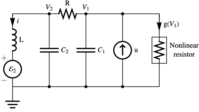
The affine model of the Chua circuit where the nonlinearity is a cubic polynomial:
pars = {Subscript[𝒞, 1] -> 1, Subscript[𝒞, 2] -> 1, ℒ -> 1, ℛ -> 1};asys = AffineStateSpaceModel[{{(-2*Subscript[𝒱, 1] - Subscript[𝒱, 1]^3 +
(-Subscript[𝒱, 1] + Subscript[𝒱, 2])/ℛ)/
Subscript[𝒞, 1],
(-𝒾 + (Subscript[𝒱, 1] - Subscript[𝒱, 2])/
ℛ)/Subscript[𝒞, 2],
(-Subscript[ℰ, 2] + Subscript[𝒱, 2])/ℒ},
{{-Subscript[𝒞, 1]^(-1)}, {0}, {0}},
{-Subscript[ℰ, 4] + Subscript[𝒱, 2]}, {{0}}},
{Subscript[𝒱, 1], Subscript[𝒱, 2], 𝒾}, Automatic,
{Automatic}, Automatic, SamplingPeriod -> None] /. pars;The exosystem, where ω is the frequency of the sinusoid to be tracked:
pars1 = {Subscript[𝒞, 1] -> 1, Subscript[𝒞, 2] -> 1, ℒ -> 1, ℛ -> 1, ω -> 10};nsys = NonlinearStateSpaceModel[
{{(-Subscript[ℰ, 1] - 2*Subscript[ℰ, 1]^3 +
(-Subscript[ℰ, 1] + Subscript[ℰ, 2])/ℛ)/
Subscript[𝒞, 1],
((Subscript[ℰ, 1] - Subscript[ℰ, 2])/ℛ -
Subscript[ℰ, 3])/Subscript[𝒞, 2],
Subscript[ℰ, 2]/ℒ, ω*Subscript[ℰ, 5],
(-ω)*Subscript[ℰ, 4]}, {}},
{Subscript[ℰ, 1], Subscript[ℰ, 2], Subscript[ℰ, 3],
Subscript[ℰ, 4], Subscript[ℰ, 5]}, {}, Automatic, Automatic,
SamplingPeriod -> None, SystemsModelLabels -> {{}, None}] /. pars1;sys = SystemsModelMerge[{asys, nsys}]The poles of the disturbance model:
Subscript[poles, d] = Eigenvalues@First@Normal@StateSpaceModel[nsys]//NThe system poles consist of the three new poles and the stabilizable poles:
decays = Join[{-1, -2, -3}, DeleteCases[%, Complex[_ ? PossibleZeroQ, _]]]k = FullInformationOutputRegulator[{sys, All, All, {7, 8}}, {"Poles", decays}]csys = SystemsModelStateFeedbackConnect[sys, k]//SimplifyThe simulation shows that the regulation is achieved:
OutputResponse[{csys, {10, 0, 0.1, 0, 0, 0, 0, -1}}, 0, {t, 0, 10}];
Plot[%, {t, 0, 10}, PlotRange -> All]
Properties & Relations (4)
StateFeedbackGains is a special case:
ssm = StateSpaceModel[{{{2, 0, -1}, {0, -2, 1}, {1, -1, 1}}, {{1, 1}, {0, 1}, {1, -1}},
  {{1, -1, 0}, {0, 1, -1}}, {{0, 0}, {0, 0}}}, SamplingPeriod -> None, SystemsModelLabels -> None];
poles = {-1, -2, -3};FullInformationOutputRegulator[ssm, {"Poles", poles}]StateFeedbackGains[ssm, poles]LQRegulatorGains is a special case:
ssm = StateSpaceModel[{{{2, 0, -1}, {0, -2, 1}, {1, -1, 1}}, {{1, 1}, {0, 1}, {1, -1}},
  {{1, -1, 0}, {0, 1, -1}}, {{0, 0}, {0, 0}}}, SamplingPeriod -> None, SystemsModelLabels -> None];
weights = {IdentityMatrix[3], IdentityMatrix[2]};FullInformationOutputRegulator[N@ssm, {"Weights", weights}]LQRegulatorGains[N@ssm, weights]Obtain the closed-loop system using SystemsModelStateFeedbackConnect:
sys = NonlinearStateSpaceModel[{{u + w + p*x, 0},
  {x}}, {x, w}, {u}, {Automatic}, Automatic,
SamplingPeriod -> None];SystemsModelStateFeedbackConnect[sys, FullInformationOutputRegulator[sys, {"Poles", {Subscript[p, f]}}]]Output regulation is achieved:
sys = StateSpaceModel[{{{2, 0, -1, 1}, {0, -2, 1, 0}, {1, -1, 1, 0}, {0, 0, 0, 0}},
  {{1, 1}, {0, 1}, {1, -1}, {0, 0}}, {{1, -1, 0, 0}, {0, 1, -1, 0}}, {{0, 0}, {0, 0}}},
SamplingPeriod -> None, SystemsModelLabels -> None];k = FullInformationOutputRegulator[sys, {"Poles", N@{-1, -2, -3}}]csys = SystemsModelStateFeedbackConnect[sys, k]OutputResponse[{csys, RandomReal[2, 4]}, 0, {t, 0, 5}];
Plot[Evaluate[%], {t, 0, 5}, PlotRange -> All]Text
Wolfram Research (2014), FullInformationOutputRegulator, Wolfram Language function, https://reference.wolfram.com/language/ref/FullInformationOutputRegulator.html.
CMS
Wolfram Language. 2014. "FullInformationOutputRegulator." Wolfram Language & System Documentation Center. Wolfram Research. https://reference.wolfram.com/language/ref/FullInformationOutputRegulator.html.
APA
Wolfram Language. (2014). FullInformationOutputRegulator. Wolfram Language & System Documentation Center. Retrieved from https://reference.wolfram.com/language/ref/FullInformationOutputRegulator.html