Wolfram Language & System Documentation Center

StateSpaceTransform

StateSpaceTransform[sys,{p,q}]

transforms the state-space model sys using the matrices p and q.

StateSpaceTransform[sys,{{x₁p₁[z],…},{z₁q₁[x],…}}]

transforms using the variable transformations {x₁p₁[z],…} and {z₁q₁[x],…}.

Details and Options

StateSpaceTransform returns a transformed model where the state variables have been transformed. The transformation can be a similarity, equivalence, or restricted equivalence transformation.
The system sys can be a standard or descriptor StateSpaceModel, AffineStateSpaceModel, or NonlinearStateSpaceModel.
For a standard StateSpaceModel[{a,b,c,d}], the original and transformed systems are related by the transformation and the corresponding equations are given by:
Typically p and q are inverses, in which case the transformation is a similarity transformation. The following defaults for p and q are used for standard StateSpaceModel transformations:
p or {p,Automatic} {p,Inverse[p]}

{Automatic,q} {Inverse[q],q}
For a descriptor StateSpaceModel[{a,b,c,d,e}], the original and transformed systems related by the transformation and the corresponding equations are given by:
Typically p and q are invertible matrices but not inverses, in which case the transformation is an equivalence transformation. The following defaults are used for descriptor StateSpaceModel transformations:
p or {p,Automatic} {p,IdentityMatrix[n]}

{Automatic,q} {IdentityMatrix[n],q}
For an AffineStateSpaceModel[{a,b,c,d},x] and NonlinearStateSpaceModel[{f,g},x,u] with j the Jacobian matrix D[p[z],{z}], the original and transformed systems are related by the transformation , and the corresponding equations are given by:
Typically p[z] and q[x] are inverses, in which case the transformation is an invertible mapping.
{{x₁->p₁[z],…},{z₁,…}} q[x] is computed if needed

{Automatic,{z₁->q[x],…}} p[z] is computed
When variable transformation matrices {p,q} are given, the resulting system is of the same type as the input. In the case of nonlinear state-space models, these are taken to represent the transformation rules {{x₁->p〚1〛.z,…},{z₁->q〚1〛.x,…}}.
When variable transformation rules {{x₁->p₁[z],…},…} are given, the resulting system is always AffineStateSpaceModel or NonlinearStateSpaceModel.
StateSpaceTransform accepts the option DescriptorStateSpace.

Examples

open all close all

Basic Examples (1)

A similarity transformation :

Wolfram Language code:

{ssm, p} = {StateSpaceModel[{{{0.5195, 0.2959}, {0.3081, 0.9136}}, {{0.0987}, {-1}}, {{1, 0}}, {{0}}}, 
 SamplingPeriod -> None, SystemsModelLabels -> None], p = (|     |    |
| --- | -- |
| 0.5 | 0  |
| 1   | -1 |)};

Wolfram Language code: StateSpaceTransform[ssm, p]

Use the matrix pair:

Wolfram Language code: StateSpaceTransform[ssm, {p, Inverse[p]}]

Scope (15)

Linear Transformations (10)

The similarity transformation :

Wolfram Language code:

StateSpaceTransform[StateSpaceModel[{{{a}}, {{b}}, {{c}}, {{d}}}, 
 SamplingPeriod -> None, SystemsModelLabels -> None], {{p}}]

Specify the matrix pair:

Wolfram Language code:

StateSpaceTransform[StateSpaceModel[{{{a}}, {{b}}, {{c}}, {{d}}}, 
 SamplingPeriod -> None, SystemsModelLabels -> None], {{{p}}, {{(1/p)}}}]

Specify the transformation as :

Wolfram Language code:

StateSpaceTransform[StateSpaceModel[{{{a}}, {{b}}, {{c}}, {{d}}}, 
 SamplingPeriod -> None, SystemsModelLabels -> None], {Automatic, {{(1/p)}}}]

The similarity transform for a descriptor system:

Wolfram Language code:

StateSpaceTransform[StateSpaceModel[{{{a}}, {{b}}, {{c}}, {{d}}, 
  {{e}}}, SamplingPeriod -> None, SystemsModelLabels -> None], {{{p}}, {{(1/p)}}}]

The equivalence transform for a descriptor system:

Wolfram Language code:

StateSpaceTransform[StateSpaceModel[{{{a}}, {{b}}, {{c}}, {{d}}, 
  {{e}}}, SamplingPeriod -> None, SystemsModelLabels -> None], {{p}}]

The corresponding matrix pair specification:

Wolfram Language code:

StateSpaceTransform[StateSpaceModel[{{{a}}, {{b}}, {{c}}, {{d}}, 
  {{e}}}, SamplingPeriod -> None, SystemsModelLabels -> None], {{{p}}, {{1}}}]

Obtain an equivalent descriptor system with the state equations premultiplied by a matrix q:

Wolfram Language code:

StateSpaceTransform[StateSpaceModel[{{{a}}, {{b}}, {{c}}, {{d}}, 
  {{e}}}, SamplingPeriod -> None, SystemsModelLabels -> None], {Automatic, {{q}}}]

The new states are essentially the old states, i.e. :

Wolfram Language code:

StateSpaceTransform[StateSpaceModel[{{{a}}, {{b}}, {{c}}, {{d}}, 
  {{e}}}, SamplingPeriod -> None, SystemsModelLabels -> None], {{{1}}, {{q}}}]

For a descriptor system, the transformation with an invertible p and q gives an equivalent system:

Wolfram Language code:

StateSpaceTransform[StateSpaceModel[{{{Subscript[a, 11], Subscript[a, 12]}, 
   {Subscript[a, 21], Subscript[a, 22]}}, 
  {{Subscript[b, 11]}, {Subscript[b, 21]}}, 
  {{Subscript[c, 11], Subscript[c, 12]}}, 
  {{Subscript[d, 11]}}, {{Subscript[e, 11], 
    Subscript[e, 12]}, {Subscript[e, 21], 
    Subscript[e, 22]}}}, SamplingPeriod -> None, SystemsModelLabels -> None], {(|     |     |
| --- | --- |
| p11 | p12 |
| p21 | p22 |), (|     |     |
| --- | --- |
| q11 | q12 |
| q21 | q22 |)}]

The original system:

Wolfram Language code:

StateSpaceTransform[%, Inverse /@ {(|     |     |
| --- | --- |
| p11 | p12 |
| p21 | p22 |), (|     |     |
| --- | --- |
| q11 | q12 |
| q21 | q22 |)}]

A noninvertible p or q gives a system with restricted equivalence:

Wolfram Language code:

StateSpaceTransform[StateSpaceModel[{{{Subscript[a, 11], Subscript[a, 12]}, 
   {Subscript[a, 21], Subscript[a, 22]}}, 
  {{Subscript[b, 11]}, {Subscript[b, 21]}}, 
  {{Subscript[c, 11], Subscript[c, 12]}}, 
  {{Subscript[d, 11]}}, {{Subscript[e, 11], 
    Subscript[e, 12]}, {Subscript[e, 21], 
    Subscript[e, 22]}}}, SamplingPeriod -> None, SystemsModelLabels -> None], {(|     |     |
| --- | --- |
| p11 | p12 |
| 0   | 0   |), (|     |   |
| --- | - |
| q11 | 0 |
| q21 | 0 |)}]

Linear discrete-time systems behave just like continuous-time systems under matrix transformations:

Wolfram Language code:

StateSpaceTransform[StateSpaceModel[{{{a}}, {{b}}, {{c}}, {{d}}}, 
 SamplingPeriod -> τ, SystemsModelLabels -> None], {{p}}]

Transform an AffineStateSpaceModel according to :

Wolfram Language code:

StateSpaceTransform[AffineStateSpaceModel[{{a[x]}, {{b[x]}}, 
  {c[x]}, {{d[x]}}}, {x}, 
 Automatic, {Automatic}, Automatic, SamplingPeriod -> None], {{p}}]

Specify the transformation in terms of the new variable z:

Wolfram Language code:

StateSpaceTransform[AffineStateSpaceModel[{{a[x]}, {{b[x]}}, 
  {c[x]}, {{d[x]}}}, {x}, 
 Automatic, {Automatic}, Automatic, SamplingPeriod -> None], {{x -> p z}, {z}}]

Specify the transformation as :

Wolfram Language code:

StateSpaceTransform[AffineStateSpaceModel[{{a[x]}, {{b[x]}}, 
  {c[x]}, {{d[x]}}}, {x}, 
 Automatic, {Automatic}, Automatic, SamplingPeriod -> None], {Automatic, {{(1/p)}}}]

Using variables:

Wolfram Language code:

StateSpaceTransform[AffineStateSpaceModel[{{a[x]}, {{b[x]}}, 
  {c[x]}, {{d[x]}}}, {x}, 
 Automatic, {Automatic}, Automatic, SamplingPeriod -> None], {{x}, {z -> (1/p)x}}]

Specify the transformation and its inverse:

Wolfram Language code:

StateSpaceTransform[AffineStateSpaceModel[{{a[x]}, {{b[x]}}, 
  {c[x]}, {{d[x]}}}, {x}, 
 Automatic, {Automatic}, Automatic, SamplingPeriod -> None], {{{p}}, {{(1/p)}}}]

Wolfram Language code:

StateSpaceTransform[AffineStateSpaceModel[{{a[x]}, {{b[x]}}, 
  {c[x]}, {{d[x]}}}, {x}, 
 Automatic, {Automatic}, Automatic, SamplingPeriod -> None], {{x -> p z}, {z -> (1/p)x}}]

Transform a NonlinearStateSpaceModel according to :

Wolfram Language code:

StateSpaceTransform[NonlinearStateSpaceModel[{{f[x, u]}, 
  {g[x, u]}}, {x}, {u}, 
 {Automatic}, Automatic, SamplingPeriod -> None], {{p}}]

In terms of the new variable z:

Wolfram Language code:

StateSpaceTransform[NonlinearStateSpaceModel[{{f[x, u]}, 
  {g[x, u]}}, {x}, {u}, 
 {Automatic}, Automatic, SamplingPeriod -> None], {{x -> p z}, {z}}]

In terms of the inverse transformation:

Wolfram Language code:

StateSpaceTransform[NonlinearStateSpaceModel[{{f[x, u]}, 
  {g[x, u]}}, {x}, {u}, 
 {Automatic}, Automatic, SamplingPeriod -> None], {{x}, {z -> (1/p)x}}]

The transformation and its inverse:

Wolfram Language code:

StateSpaceTransform[NonlinearStateSpaceModel[{{f[x, u]}, 
  {g[x, u]}}, {x}, {u}, 
 {Automatic}, Automatic, SamplingPeriod -> None], {{x -> p z}, {z -> (1/p)x}}]

For orthogonal matrices, Transpose can be used instead of Automatic or Inverse:

Wolfram Language code:

p = (|             |              |
| ----------- | ------------ |
| (1/Sqrt[2]) | (1/Sqrt[2])  |
| (1/Sqrt[2]) | -(1/Sqrt[2]) |);

Wolfram Language code: p.p//MatrixForm

Wolfram Language code:

StateSpaceTransform[StateSpaceModel[{{{Subscript[a, 1, 1], Subscript[a, 1, 2]}, 
   {Subscript[a, 2, 1], Subscript[a, 2, 2]}}, 
  {{Subscript[b, 1, 1]}, {Subscript[b, 2, 1]}}, 
  {{Subscript[c, 1, 1], Subscript[c, 1, 2]}}, 
  {{Subscript[d, 1, 1]}}}, SamplingPeriod -> None, SystemsModelLabels -> None], {p, p}]

Nonlinear Transformations: (5)

Nonlinear transformations of a StateSpaceModel:

Wolfram Language code:

StateSpaceTransform[StateSpaceModel[{{{a}}, {{b}}, {{c}}, {{d}}}, 
 SamplingPeriod -> None, SystemsModelLabels -> None], {{x -> p[z]}, {z}}]

Wolfram Language code:

StateSpaceTransform[StateSpaceModel[{{{a}}, {{b}}, {{c}}, {{d}}}, 
 SamplingPeriod -> None, SystemsModelLabels -> None], {{x}, {z -> q[x]}}]

Nonlinear transformations of an AffineStateSpaceModel:

Wolfram Language code:

StateSpaceTransform[AffineStateSpaceModel[{{a[x]}, {{b[x]}}, 
  {c[x]}, {{d[x]}}}, {x}, 
 Automatic, {Automatic}, Automatic, SamplingPeriod -> None], {{x -> p[z]}, {z}}]

Wolfram Language code:

StateSpaceTransform[AffineStateSpaceModel[{{a[x]}, {{b[x]}}, 
  {c[x]}, {{d[x]}}}, {x}, 
 Automatic, {Automatic}, Automatic, SamplingPeriod -> None], {{x}, {z -> q[x]}}]

Nonlinear transformations of a NonlinearStateSpaceModel:

Wolfram Language code:

StateSpaceTransform[NonlinearStateSpaceModel[{{f[x, u]}, 
  {g[x, u]}}, {x}, {u}, 
 {Automatic}, Automatic, SamplingPeriod -> None], {{x -> p[z]}, {z}}]

Wolfram Language code:

StateSpaceTransform[NonlinearStateSpaceModel[{{f[x, u]}, 
  {g[x, u]}}, {x}, {u}, 
 {Automatic}, Automatic, SamplingPeriod -> None], {{x}, {z -> q[x]}}]

Specify a nonlinear transformation and its inverse:

Wolfram Language code:

StateSpaceTransform[StateSpaceModel[{{{Subscript[a, 1, 1], Subscript[a, 1, 2]}, 
   {Subscript[a, 2, 1], Subscript[a, 2, 2]}}, 
  {{Subscript[b, 1, 1]}, {Subscript[b, 2, 1]}}, 
  {{Subscript[c, 1, 1], Subscript[c, 1, 2]}}, 
  {{Subscript[d, 1, 1]}}}, SamplingPeriod -> None, SystemsModelLabels -> None], {{Subscript[x, 1] -> Subscript[z, 1] + Subscript[z, 1]Subscript[z, 1], Subscript[x, 2] -> Subscript[z, 2] + Subscript[z, 1]}, {Subscript[z, 1] -> (1/2) (-1 + Sqrt[1 + 4 Subscript[x, 1]]), Subscript[z, 2] -> (1/2) (1 - Sqrt[1 + 4 Subscript[x, 1]] + 2 Subscript[x, 2])}}]

The inverse of a nonlinear transformation is required only if operating points are specified:

Wolfram Language code:

StateSpaceTransform[AffineStateSpaceModel[{{a[x]}, {{b[x]}}, 
  {c[x]}, {{d[x]}}}, 
 {{x, Subscript[x, 0]}}, Automatic, {Automatic}, Automatic, 
 SamplingPeriod -> None], {{x -> p z}, {z -> (1/p)x}}]

Generalizations & Extensions (2)

A non-square orthogonal matrix selects a subsystem:

Wolfram Language code:

ssm = StateSpaceModel[{{{Subscript[a, 1], 0, 0}, {0, Subscript[a, 2], 0}, 
   {0, 0, Subscript[a, 3]}}, {{0, 0}, {Subscript[b, 1], 0}, 
   {0, Subscript[b, 2]}}, {{Subscript[c, 1], 0, 0}, 
   {0, 0, Subscript[c, 3]}}, 
  {{Subscript[d, 11], Subscript[d, 12]}, 
   {Subscript[d, 21], Subscript[d, 22]}}}, SamplingPeriod -> None, 
 SystemsModelLabels -> None];

Wolfram Language code: p = {{0, 0}, {1, 0}, {0, 1}};

Wolfram Language code: StateSpaceTransform[ssm, p]

The corresponding matrix pair:

Wolfram Language code: StateSpaceTransform[ssm, {p, p}]

For nonlinear transformations, a partitioned inverse specification selects a subsystem:

Wolfram Language code:

assm = AffineStateSpaceModel[{{Subscript[a, 1]*Subscript[x, 1], 
   Subscript[a, 2]*Subscript[x, 2], 
   Subscript[a, 3]*Subscript[x, 3]}, 
  {{Subscript[b, 1]}, {Subscript[b, 2]}, {Subscript[b, 3]}}, 
  {Subscript[c, 1]*Subscript[x, 1], 
   Subscript[c, 2]*Subscript[x, 2]}, 
  {{Subscript[d, 1]}, {Subscript[d, 2]}}}, 
 {Subscript[x, 1], Subscript[x, 2], Subscript[x, 3]}, 
 Automatic, {Automatic, Automatic}, Automatic, SamplingPeriod -> None];
pp = {Subscript[x, 1] -> Subscript[z, 1], Subscript[x, 2] -> Subscript[z, 2], Subscript[x, 3] -> Subscript[z, 3]};
qq = {{Subscript[z, 1] -> Subscript[x, 1], Subscript[z, 2] -> Subscript[x, 2]}, {Subscript[z, 3] -> Subscript[x, 3]}};

Wolfram Language code: StateSpaceTransform[assm, {pp, qq}]

The complete system:

Wolfram Language code: StateSpaceTransform[assm, {pp, Flatten[qq]}]

Options (1)

DescriptorStateSpace (1)

Treat a standard StateSpaceModel as a descriptor system:

Wolfram Language code:

StateSpaceTransform[StateSpaceModel[{{{a}}, {{b}}, {{c}}, {{d}}}, 
 SamplingPeriod -> None, SystemsModelLabels -> None], {{p}}, DescriptorStateSpace -> True]

It gives the same result as an explicit descriptor specification:

Wolfram Language code:

StateSpaceTransform[StateSpaceModel[{{{a}}, {{b}}, {{c}}, {{d}}, 
  {{1}}}, SamplingPeriod -> None, SystemsModelLabels -> None], {{p}}]

Similar results can be obtained with the inverse transformation as well:

Wolfram Language code:

StateSpaceTransform[StateSpaceModel[{{{a}}, {{b}}, {{c}}, {{d}}}, 
 SamplingPeriod -> None, SystemsModelLabels -> None], {Automatic, {{q}}}, DescriptorStateSpace -> True]

Wolfram Language code:

StateSpaceTransform[StateSpaceModel[{{{a}}, {{b}}, {{c}}, {{d}}, 
  {{1}}}, SamplingPeriod -> None, SystemsModelLabels -> None], {Automatic, {{q}}}]

Applications (6)

A function to obtain the controllable companion form of a single-input system:

Wolfram Language code:

ControllableCompanion[ssm_StateSpaceModel] /; ControllableModelQ[ssm] := Module[{A = First@Normal@ssm, dim, cv, coeffsList, mat, s1}, 
	dim = Last@Dimensions@A;
	coeffsList = CoefficientList[Det[cv IdentityMatrix[dim] - A], cv];
	mat = HankelMatrix[Rest[coeffsList] / Last[coeffsList]];
	s1 = ControllabilityMatrix[ssm].mat;
	StateSpaceTransform[ssm, s1]]

Wolfram Language code:

ControllableCompanion[StateSpaceModel[{{{1, -1, 1}, {1, 2, 1}, {-1, 1, 2}}, {{1}, {-1}, {0}}, {{1, -1, 0}}, {{0}}}, 
 SamplingPeriod -> None, SystemsModelLabels -> None]]

A function to obtain the observable companion form of a single-output system:

Wolfram Language code:

ObservableCompanion[ssm_StateSpaceModel] /; ObservableModelQ[ssm] := Module[{A = First@Normal@ssm, dim, cv, coeffsList, mat, s1}, 
	dim = Last@Dimensions@A;
	coeffsList = CoefficientList[Det[cv IdentityMatrix[dim] - A], cv];
	mat = HankelMatrix[Rest[coeffsList] / Last[coeffsList]];
	s1 = mat.ObservabilityMatrix[ssm];
	StateSpaceTransform[ssm, {Inverse@s1, s1}]]

Wolfram Language code:

ObservableCompanion[StateSpaceModel[{{{1, -1, 1}, {1, 2, 1}, {-1, 1, 2}}, {{1}, {-1}, {0}}, {{1, -1, 0}}, {{0}}}, 
 SamplingPeriod -> None, SystemsModelLabels -> None]]

Rearrange the states:

Wolfram Language code:

ssm = StateSpaceModel[{{{Subscript[a, 11], Subscript[a, 12], 
    Subscript[a, 13], Subscript[a, 14]}, 
   {Subscript[α, 21], Subscript[α, 22], Subscript[α, 23], 
    Subscript[α, 24]}, {Subscript[Α, 31], 
    Subscript[Α, 32], Subscript[Α, 33], 
    Subscript[Α, 34]}, {Subscript[a, 41], Subscript[a, 42], 
    Subscript[a, 43], Subscript[a, 44]}}, 
  {{Subscript[b, 1]}, {Subscript[β, 2]}, 
   {Subscript[Β, 3]}, {Subscript[b, 4]}}, 
  {{Subscript[c, 11], Subscript[γ, 12], Subscript[Γ, 13], 
    Subscript[c, 14]}, {Subscript[c, 21], Subscript[γ, 22], 
    Subscript[Γ, 23], Subscript[c, 24]}}, 
  {{Subscript[d, 1]}, {Subscript[d, 2]}}}, SamplingPeriod -> None, 
 SystemsModelLabels -> None];

Wolfram Language code:

StateSpaceTransform[ssm, (|   |   |   |   |
| - | - | - | - |
| 1 | 0 | 0 | 0 |
| 0 | 0 | 1 | 0 |
| 0 | 1 | 0 | 0 |
| 0 | 0 | 0 | 1 |)]

Convert the model of a simple pendulum in Cartesian coordinates to polar coordinates:

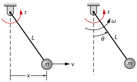
The model in Cartesian coordinates:

Wolfram Language code:

asys = AffineStateSpaceModel[
 {{v, (-v^2)*(x/(L^2 - x^2)) - 
    (g*x*Sqrt[L^2 - x^2])/L^2}, 
  {{0}, {Sqrt[L^2 - x^2]/(L^2*m)}}, 
  {ArcSin[x/L]}, {{0}}}, {x, v}, 
 {τ}, {Automatic}, Automatic, SamplingPeriod -> None];

The model in polar coordinates:

Wolfram Language code: StateSpaceTransform[asys, {{x -> L Sin[θ], v -> L Cos[θ] ω}, {θ, ω}}]//PowerExpand

Apply a direct quadrature (dq) transformation to a permanent magnet stepper motor model: »

Wolfram Language code:

motor = AffineStateSpaceModel[{{((-R)*Subscript[i, a] + 
     ω*Sin[θ*Subscript[n, r]]*
      Subscript[K, m])/L, 
   ((-R)*Subscript[i, b] - 
     ω*Cos[θ*Subscript[n, r]]*
      Subscript[K, m])/L, 
   ((-b)*ω - 
     Sin[θ*Subscript[n, r]]*
      Subscript[i, a]*Subscript[K, m] + 
     Cos[θ*Subscript[n, r]]*
      Subscript[i, b]*Subscript[K, m])/J, 
   ω}, {{1, 0}, {0, 1}, {0, 0}, {0, 0}}, {θ, ω}, 
  {{0, 0}, {0, 0}}}, {Subscript[i, a], 
  Subscript[i, b], ω, θ}, 
 {Subscript[v, a], Subscript[v, b]}, 
 {Automatic, Automatic}, Automatic, SamplingPeriod -> None];

Apply the dq transformation to the currents and :

Wolfram Language code:

StateSpaceTransform[motor, {{Subscript[i, a] -> Subscript[i, d] Cos[Subscript[n, r]θ] - Subscript[i, q] Sin[Subscript[n, r]θ], Subscript[i, b] -> Subscript[i, d] Sin[Subscript[n, r]θ] + Subscript[i, q] Cos[Subscript[n, r]θ], ω -> ω, θ -> θ}, {Subscript[i, d], Subscript[i, q], ω, θ}}]

Apply the dq transformation to the input voltages as well:

Wolfram Language code:

SystemsModelSeriesConnect[TransferFunctionModel[{{{Cos[θ*Subscript[n, r]], 
    -Sin[θ*Subscript[n, r]]}, 
   {Sin[θ*Subscript[n, r]], 
    Cos[θ*Subscript[n, r]]}}, 1}, ], %]//Simplify

Convert aircraft equations of motion from body to wind coordinates:

Wolfram Language code:

nsys = NonlinearStateSpaceModel[{{r*v - q*w + 
    X/m - g*Sin[θ], 
   (-r)*u + p*w + 
    Y/m + g*Cos[θ]*Sin[ϕ], 
   q*u - p*v + Z/m + 
    g*Cos[θ]*Cos[ϕ]}, {}}, 
 {u, v, w}, {X, Y, 
  Z}, Automatic, Automatic, SamplingPeriod -> None, SystemsModelLabels -> {{}, None}];

Wolfram Language code: Simplify[StateSpaceTransform[nsys, {{u -> V Cos[α] Cos[β], v -> V Sin[β], w -> V Sin[α] Cos[β]}, {V, α, β}}]]

Properties & Relations (8)

The output response is invariant under a similarity transformation:

Wolfram Language code:

ssm1 = StateSpaceModel[{{{-0.75, 0.25}, {-0.01, -1}}, {{0.005}, {0.05}}, {{1, 0}}, {{0}}}, 
 SamplingPeriod -> None, SystemsModelLabels -> None];
ssm2 = StateSpaceTransform[ssm1, {{1, -1}, {0, 1}}];

Wolfram Language code:

Grid[{Table[Plot[Evaluate@OutputResponse[s, 1, {t, 10}], {t, 0, 10}, ImageSize -> Small], {s, {ssm1, ssm2}}]}, Spacings -> 2]

Similar systems have identical transfer functions:

Wolfram Language code:

ssm1 = StateSpaceModel[{{{a}}, {{b}}, {{c}}, {{d}}}, 
 SamplingPeriod -> None, SystemsModelLabels -> None];
ssm2 = StateSpaceTransform[ssm1, {{p}}];

Wolfram Language code: TransferFunctionModel[ssm1][s] == TransferFunctionModel[ssm2][s]

The eigenvalues (and hence, stability) are invariant under a similarity transformation:

Wolfram Language code:

ssm1 = StateSpaceModel[{{{Subscript[a, 11], Subscript[a, 12]}, 
   {Subscript[a, 21], Subscript[a, 22]}}, 
  {{Subscript[b, 1]}, {Subscript[b, 2]}}, 
  {{Subscript[c, 1], Subscript[c, 2]}}, {{0}}}, SamplingPeriod -> None, 
 SystemsModelLabels -> None];
ssm2 = StateSpaceTransform[ssm1, {{Subscript[p, 11], Subscript[p, 12]}, {Subscript[p, 21], Subscript[p, 22]}}];

Wolfram Language code: {a1, a2} = First /@ Normal /@ {ssm1, ssm2};

Wolfram Language code: Simplify[Eigenvalues[a1] == Eigenvalues[a2]]

Controllability and observability are invariant under a similarity transformation:

Wolfram Language code:

ssm1 = StateSpaceModel[{{{Subscript[a, 11], 0}, {0, Subscript[a, 22]}}, 
  {{Subscript[b, 1]}, {0}}, 
  {{Subscript[c, 1], Subscript[c, 2]}}, {{0}}}, SamplingPeriod -> None, 
 SystemsModelLabels -> None];
ssm2 = StateSpaceTransform[ssm1, {{Subscript[p, 11], Subscript[p, 12]}, {Subscript[p, 21], Subscript[p, 22]}}];

Wolfram Language code: ControllableModelQ /@ {ssm1, ssm2}

Wolfram Language code: ObservableModelQ /@ {ssm1, ssm2}

The Hankel singular values are invariant under similarity transformation:

Wolfram Language code:

hankelSingularValues[sys_] := 
	Module[{ns = N[sys]}, wc = ControllabilityGramian[ns];wo = ObservabilityGramian[ns];Sqrt[Eigenvalues[wc.wo]]];

Wolfram Language code:

ssm1 = StateSpaceModel[{{{-1, 0, 3}, {2, -1, 3}, {1, -1, -1}}, {{1}, {1}, {2}}, {{0, 1, -1}}, {{0}}}, 
 SamplingPeriod -> None, SystemsModelLabels -> None];
ssm2 = StateSpaceTransform[ssm1, {{1, -1, 1}, {0, 1, 0}, {1, 0, 0}}];

Wolfram Language code: hankelSingularValues[ssm1] - hankelSingularValues[ssm2]//Norm

Systems model decompositions all use state transformations:

Wolfram Language code:

ssm = StateSpaceModel[{{{0, 1}, {-12, -7}}, {{0}, {1}}, {{2, 1}}, {{0}}}, SamplingPeriod -> None, 
 SystemsModelLabels -> None];

ControllableDecomposition based on ControllabilityMatrix:

Wolfram Language code:

{p, ssmt} = ControllableDecomposition[ssm];
{StateSpaceTransform[ssm, p], ssmt}

ObservableDecomposition based on ObservabilityMatrix:

Wolfram Language code:

{p, ssmt} = ObservableDecomposition[ssm];
{StateSpaceTransform[ssm, p], ssmt}

InternallyBalancedDecomposition based on ObservabilityGramian:

Wolfram Language code:

{p, ssmt} = InternallyBalancedDecomposition[ssm];
{StateSpaceTransform[ssm, p], ssmt}//N

JordanModelDecomposition based on JordanDecomposition:

Wolfram Language code:

{p, ssmt} = JordanModelDecomposition[ssm];
{StateSpaceTransform[ssm, p], ssmt}

KroneckerModelDecomposition:

Wolfram Language code:

{p, ssmt} = KroneckerModelDecomposition[ssm];
{StateSpaceTransform[ssm, p], ssmt}

The linearization using coordinate transformations is also related using StateSpaceTransform:

Wolfram Language code:

𝒮 = StateTransformationLinearize[asys = AffineStateSpaceModel[{{4*Subscript[x, 1], 7*Subscript[x, 1]^2 + 
    Subscript[x, 2]}, {{1}, {-1 + 2*Subscript[x, 1]}}, 
  {Subscript[x, 1]}, {{0}}}, {Subscript[x, 1], 
  Subscript[x, 2]}, {{Subscript[, 1], 0}}, {Automatic}, Automatic, 
 SamplingPeriod -> None]];

Wolfram Language code: {StateSpaceTransform[asys, 𝒮[{"StateTransformation", "InverseStateTransformation"}]], 𝒮["TransformedSystem"]}

A state transformation is an intermediate step in feedback linearization:

Wolfram Language code:

asys = AffineStateSpaceModel[{{Subscript[x, 2] + Subscript[x, 2]^2, 
   Subscript[x, 3] - Subscript[x, 1]*Subscript[x, 4] + 
    Subscript[x, 4]*Subscript[x, 5], 
   -Subscript[x, 2]^2 + Subscript[x, 2]*Subscript[x, 4] + 
    Subscript[x, 1]*Subscript[x, 5], Subscript[x, 5], 
   Subscript[x, 2]^2}, {{0, 1}, {0, 0}, 
   {Cos[Subscript[x, 1] - Subscript[x, 5]], 1}, {0, 0}, {0, 1}}, 
  {Subscript[x, 1] - Subscript[x, 5], Subscript[x, 4]}, 
  {{0, 0}, {0, 0}}}, {Subscript[x, 1], Subscript[x, 2], 
  Subscript[x, 3], Subscript[x, 4], Subscript[x, 5]}, 
 {Subscript[u, 1], Subscript[u, 2]}, {Automatic, Automatic}, Automatic, 
 SamplingPeriod -> None];
ℱ = FeedbackLinearize[asys]

Apply the feedback and then the state transformation to get the transformed system:

Wolfram Language code: SystemsModelSeriesConnect[ℱ["FeedbackCompensator"], asys];

Wolfram Language code: StateSpaceTransform[%, {Automatic, ℱ["InverseStateTransformation"]}]

The property "TransformedSystem" gives the same result:

Wolfram Language code: NonlinearStateSpaceModel[ℱ["TransformedSystem"]]

Possible Issues (2)

The transformation matrix must be orthonormal or invertible:

Wolfram Language code: p = {{2, 1, 1}, {1, 0, -1}, {1, 1, 2}};

Wolfram Language code: StateSpaceTransform[StateSpaceModel[{RandomReal[2, {3, 3}], RandomReal[1, {3, 1}], {{1, 0, 0}}}], p]

It is neither orthonormal nor invertible:

Wolfram Language code: {p.p == IdentityMatrix[3], MatrixRank[p] == 3}

If there are multiple inverse solutions, only one is chosen:

Wolfram Language code:

assm = AffineStateSpaceModel[{{-Subscript[x, 1] + Subscript[x, 2], 
   -Subscript[x, 1]}, {{1 + Subscript[x, 2]}, 
   {Subscript[x, 1]}}, {Subscript[x, 1]}, {{0}}}, 
 {{Subscript[x, 1], 0}, {Subscript[x, 2], 0}}, Automatic, {Automatic}, 
 Automatic, SamplingPeriod -> None];

Wolfram Language code:

pp = {Subscript[x, 1] -> Subscript[z, 1] + Subsuperscript[z, 2, 2], Subscript[x, 2] -> Subscript[z, 2] + Subscript[z, 1]Subscript[z, 2]};
qq = {Subscript[z, 1], Subscript[z, 2]};

Wolfram Language code: StateSpaceTransform[assm, {pp, qq}]

There are 3 inverse solutions:

Wolfram Language code:

sols = Solve[Equal@@@pp, qq];
Length[sols]

Choose a desired inverse:

Wolfram Language code: StateSpaceTransform[assm, {pp, sols[[3]]}]

Top

More Learning

Tech Support

Wolfram Solutions

Wolfram Solutions For Education

Get Started

Grow Your Skills

Work with Us

Educational Programs for Adults

Educational Programs for Youth

Read

StateSpaceTransform

Details and Options

Examples

Basic Examples (1)

Scope (15)

Linear Transformations (10)

Nonlinear Transformations: (5)

Generalizations & Extensions (2)

Options (1)

DescriptorStateSpace (1)

Applications (6)

Properties & Relations (8)

Possible Issues (2)

Text

CMS

APA

BibTeX

BibLaTeX

	p or {p,Automatic}	{p,Inverse[p]}
	{Automatic,q}	{Inverse[q],q}

	p or {p,Automatic}	{p,IdentityMatrix[n]}
	{Automatic,q}	{IdentityMatrix[n],q}

	{{x₁->p₁[z],…},{z₁,…}}	q[x] is computed if needed
	{Automatic,{z₁->q[x],…}}	p[z] is computed

StateSpaceTransform

Details and Options

Examples

Basic Examples (1)

Scope (15)

Linear Transformations (10)

Nonlinear Transformations: (5)

Generalizations & Extensions (2)

Options (1)

DescriptorStateSpace (1)

Applications (6)

Properties & Relations (8)

Possible Issues (2)

See Also

Related Guides

History

Text

CMS

APA

BibTeX

BibLaTeX