HardcorePointProcess[μ,rh,d]
represents a hard-core point process with constant intensity μ and hard-core radius rh in ![]() .
.


HardcorePointProcess
HardcorePointProcess[μ,rh,d]
represents a hard-core point process with constant intensity μ and hard-core radius rh in ![]() .
.
Details
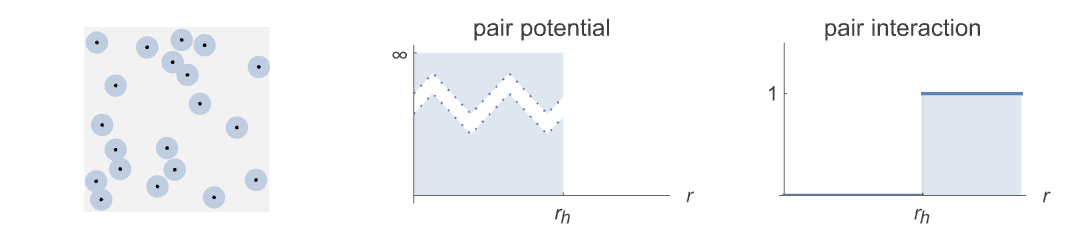
- HardcorePointProcess models point configurations where the points cannot be within a radius rh of each other but otherwise are uniformly distributed with intensity μ points per volume unit.
- The hard-core model is typically used when the underlying points behave like a collection of hard marbles, including things like gas molecules, metal deposits, sintered material and biological cells.
- The hard-core point process can be defined as a GibbsPointProcess in terms of its intensity μ and the pair potential
 or pair interaction
  , which are both parametrized by rh as follows:
 -

pair potential 
pair interaction - A point configuration
 from a hard-core point process HardcorePointProcess[μ,rh,d] in an observation region reg has density function
  proportional to
 ![mu^n product_(i!=j)Boole[||p_i-p_j||>r_(h)]](Files/HardcorePointProcess.en/9.png "mu^n product_(i!=j)Boole[||p_i-p_j||>r_(h)]") with respect to PoissonPointProcess[1,d].
with respect to PoissonPointProcess[1,d]. - The Papangelou conditional density
 for adding a point
  to a point configuration
  is
is ![mu product_iBoole[||p_i-q||>r_(h)]](Files/HardcorePointProcess.en/13.png "mu product_iBoole[||p_i-q||>r_(h)]") .
. - HardcorePointProcess allows μ and rh to be any positive numbers, and d to be any positive integer.
- HardcorePointProcess is a special case of GibbsPointProcess and is equivalent to StraussPointProcess[μ, 0, rh].
- Possible Method settings in RandomPointConfiguration for HardcorePointProcess are:
-
"MCMC" MCMC birth and death "Exact" coupling from the past - Possible PointProcessEstimator settings in EstimatedPointProcess for HardcorePointProcess are:
-
Automatic automatically choose the parameter estimator "MaximumPseudoLikelihood" maximize the pseudo-likelihood - HardcorePointProcess can be used with such functions as RipleyK and RandomPointConfiguration.
Examples
open all close allBasic Examples (2)
Sample from a hard-core point process in ![]() :
:
proc = HardcorePointProcess[30, 0.3, 2];reg = Rectangle[{0, 0}, {10, 10}];pts = RandomPointConfiguration[proc, reg]Visualize the points in the sample:
ListPlot[pts]Sample from a hard-core point process defined on the surface of the Earth:
reg = Entity["Country", "Switzerland"]["Polygon"]pts = RandomPointConfiguration[HardcorePointProcess[Quantity[3/1000, 1/"Kilometers"^2], Quantity[3, "Kilometers"], 2], reg]GeoListPlot[pts]Scope (3)
Generate three realizations from a hard-core point process in ![]() :
:
proc = HardcorePointProcess[10, 0.1, 2];reg = Disk[];pts = RandomPointConfiguration[proc, reg, 3]ListPlot[pts]Clear[μ, r, d];EstimatedPointProcess[pts, HardcorePointProcess[μ, r, d]]Generate three realizations from a hard-core point process on the surface of the Earth:
μ = Quantity[10. ^ -2, "Kilometers" ^ -2];
r = Quantity[5., "Kilometers"];proc = HardcorePointProcess[μ, r, 2];
reg = GeoDisk[Entity["City", {"SaintPetersburg", "SaintPetersburg", "Russia"}], Quantity[20, "Kilometers"]];pts = RandomPointConfiguration[proc, reg, 2]Visualize the point configurations:
GeoListPlot[pts]Clear[μ, r, d];
EstimatedPointProcess[pts, HardcorePointProcess[μ, r, d]]Generate samples with increasing hard-core radius:
proc[r_] := HardcorePointProcess[30, r, 2];sample[r_] := RandomPointConfiguration[proc[r], Rectangle[{0, 0}, {10, 10}]];range = {.3, 1, 2};Table[ListPlot[sample[r], PlotLabel -> Row[{"r = ", r}]], {r, range}]Plot samples with the repulsion disks:
HardcoreDisk[data_, r_] :=
Show[Graphics[{Opacity[0.5], LightBlue, EdgeForm[LightGray], Map[Disk[#, r]&, data["Points"]]}], ListPlot[data]]Table[Labeled[HardcoreDisk[sample[r], r], Row[{"r = ", r}]], {r, range}]Check that the hard-core constraint is obeyed:
pairWiseDists[pts_] := Block[{tp = pts}, Table[EuclideanDistance[pt, #]& /@ (tp = Rest[tp]), {pt, Most[pts]}]]Table[Min[pairWiseDists[sample[r]["Points"]]], {r, range}]Thread[% > range]Options (4)
Method (4)
Simulate using the Markov chain Monte Carlo method:
proc = HardcorePointProcess[100, .01, 2];
reg = Disk[];RandomPointConfiguration[proc, reg, Method -> "MCMC"]Specify the number of recursive calls to the sampler:
RandomPointConfiguration[proc, reg, Method -> {"MCMC", MaxRecursion -> 6}]RandomPointConfiguration[proc, reg, Method -> {"MCMC", "LengthOfRun" -> 5 * 10 ^ 4}]Provide an initial state for the simulation:
proc = HardcorePointProcess[50, rHC = 0.3, 2];
reg = Disk[];pts1 = RandomPointConfiguration[proc, reg, Method -> {"MCMC", "InitialState" -> {{1, 0}, {0, 1}}}]The initial point must have nonzero density to ensure that the result is a valid configuration:
minDistance[pts_] := Min@Nearest[pts -> "Distance", pts, 2][[All, 2]]
init = RandomPoint[reg, 100];minDistance[init] > rHCpts2 = RandomPointConfiguration[proc, reg, Method -> {"MCMC", "InitialState" -> init, "LengthOfRun" -> 10}]Check if the minimal distance between the points is smaller than the hard-core radius:
minDistance[pts2["Points"]] > rHCminDistance[pts1["Points"]] > rHCVisualize the birth and death process at different stages:
proc = HardcorePointProcess[50, rHC = 0.3, 2];
reg = Disk[];path = Table[
BlockRandom[
SeedRandom[1];
RandomPointConfiguration[proc, reg, Method -> {"MCMC", "InitialState" -> {{0., 0.4}, {-0.3, -0.2}}, "LengthOfRun" -> len}]["Points"]]
, {len, 1, 100}];Animate[
Graphics[{Lighter[GrayLevel[.4], .8], Disk[{0, 0}, 1.02], Black, PointSize[0.02], Point[path[[i]]]}]
, {i, 1, Length[path], 1}, TrackedSymbols :> i, SaveDefinitions -> True, AnimationRate -> 2, AnimationRunning -> False]Use coupling from the past for exact sampling:
proc = HardcorePointProcess[8, 0.3, 2];SeedRandom[0];pts = RandomPointConfiguration[proc, Rectangle[{0, 0}, {5, 5}], Method -> "Exact"]ListPlot[pts]Properties & Relations (3)
For the large intensity μ, the samples saturate:
proc[μ_] := HardcorePointProcess[μ, .3, 2];reg = Rectangle[{0, 0}, {10, 10}];intensities = {1, 5, 10, 100, 300, 500};samples = Table[Quiet@RandomPointConfiguration[proc[μ], reg], {μ, intensities}];ListPlot[#, PlotLabel -> #["PointCount"]]& /@ samplesThe number of points saturates at a density that is significantly lower than the theoretical maximum packing:
reg  = Rectangle[{0, 0}, {10, 10}];
r = .3;pts = RandomPointConfiguration[HardcorePointProcess[300, r, 2], reg, Method -> {"MCMC", "LengthOfRun" -> 1000}];pts["PointCount"](RegionMeasure[reg]/2 Sqrt[3](r / 2)^2)pts["PointCount"](r / 2)^2π / RegionMeasure[reg]reg = Cuboid[{0, 0, 0}];
r = .1;pts = RandomPointConfiguration[HardcorePointProcess[3000, r, 3], reg, Method -> {"MCMC", "LengthOfRun" -> 1000}];pts["PointCount"]RegionMeasure[reg](Sqrt[2]/r^3)pts["PointCount"] * RegionMeasure[Ball[{0, 0, 0}, r / 2]] / RegionMeasure[reg]Compute the average number of points in a unit disk for a hard-core point process:
𝒟 = PointCountDistribution[HardcorePointProcess[20, .5, 2], Disk[]];NExpectation[n, n𝒟, Method -> {"MonteCarlo", "SamplingIncrement" -> 10 ^ 4}]Possible Issues (1)
By default, the simulation will run until the number of points converges to a steady state, or until the default number of iterations is reached:
proc = HardcorePointProcess[10 ^ 3, .0001, 2];
reg = Disk[];RandomPointConfiguration[proc, reg]Raise the number of recursive calls to the sampler:
RandomPointConfiguration[proc, reg, Method -> {"MCMC", MaxRecursion -> 6}]RandomPointConfiguration[proc, reg, Method -> {"MCMC", "LengthOfRun" -> 5 * 10 ^ 4}]Text
Wolfram Research (2020), HardcorePointProcess, Wolfram Language function, https://reference.wolfram.com/language/ref/HardcorePointProcess.html.
CMS
Wolfram Language. 2020. "HardcorePointProcess." Wolfram Language & System Documentation Center. Wolfram Research. https://reference.wolfram.com/language/ref/HardcorePointProcess.html.
APA
Wolfram Language. (2020). HardcorePointProcess. Wolfram Language & System Documentation Center. Retrieved from https://reference.wolfram.com/language/ref/HardcorePointProcess.html