HilbertCurve[n]
gives the line segments representing the n![]() -step Hilbert curve.
-step Hilbert curve.
HilbertCurve[n,d]
gives the n![]() -step Hilbert curve in dimension d.
-step Hilbert curve in dimension d.


HilbertCurve
HilbertCurve[n]
gives the line segments representing the n![]() -step Hilbert curve.
-step Hilbert curve.
HilbertCurve[n,d]
gives the n![]() -step Hilbert curve in dimension d.
-step Hilbert curve in dimension d.
Details and Options
- HilbertCurve is also known as Hilbert space-filling curve.
- HilbertCurve[n] returns a Line primitive corresponding to a path that starts at {0,0}, then joins all integer points in the 2n-1 by 2n-1 square, and ends at {2n-1,0}. »
- HilbertCurve takes a DataRange option that can be used to specify the range the coordinates should be assumed to occupy.
Examples
open all close allBasic Examples (2)
Graphics[HilbertCurve[2]]Lengths of the approximations to the Hilbert curve:
Table[RegionMeasure[HilbertCurve[n]], {n, 5}]//RationalizeFindSequenceFunction[%, n]Visualize the Hilbert curve in 2D with splines:
Graphics[{Thickness[Large], HilbertCurve[4] /. Line -> BSplineCurve}]Scope (8)
Curve Specification (4)
Curve Styling (4)
Hilbert curves with different thicknesses:
Table[Region[HilbertCurve[4], BaseStyle -> {Thickness[i]}], {i, {Medium, Large}}]Table[Graphics[{Thickness[i], HilbertCurve[4]}], {i, {Medium, Large}}]Table[Graphics[{Thickness[i], HilbertCurve[3]}], {i, {.005, .05, .1}}]Thickness in printer's points:
Table[Graphics[{AbsoluteThickness[i], HilbertCurve[3]}], {i, {1, 5, 10}}]Table[Graphics[{Dashing[i], HilbertCurve[4]}], {i, {Tiny, Small, Medium, Large}}]Table[Graphics[{d, HilbertCurve[4]}], {d, {Dotted, Dashed, DotDashed}}]Table[Graphics[{c, HilbertCurve[4]}], {c, {Red, Green, Blue, Yellow}}]Generalizations & Extensions (2)
Options (1)
DataRange (1)
DataRange allows you to specify the range of mesh coordinates to generate:
HilbertCurve[2, 2]HilbertCurve[2, 2, DataRange -> {{0, 1}, {0, 1}}]Applications (4)
HilbertCurve is constructed recursively by transforming cups into four cups linked together by lines:
cups[curve_] := With[{part = Partition[First[curve], UpTo[5], 4]},
Graphics[Apply[{{Thick, Line[#1]}, {Dashed, Line[#2]}}&, Map[Partition[#, UpTo[4], 3]&, part], {1}]]]Row[{cups[HilbertCurve[1]], cups[HilbertCurve[2]]}, Spacer[40]]color[curve_, n_ : 1] := With[{color = ColorData[97, "ColorList"], data = First[cups[curve]]},
Graphics[MapIndexed[{color[[First[#2]]], #1}&, Partition[data, n]]]]Row[{color[HilbertCurve[2]], color[HilbertCurve[3], 4]}, Spacer[40]]Visualize the Hilbert curve in 2D:
Graphics[HilbertCurve[4]]% /. Line -> BSplineCurveGraphics3D[HilbertCurve[3, 3]]% /. Line -> TubeBuild a polygon from the Hilbert curve:
Graphics[Polygon @@ HilbertCurve[5]]Apply a Hilbert curve texture to a surface:
ParametricPlot3D[{1.16 ^ v Cos[v](1 + Cos[u]), -1.16 ^ v Sin[v](1 + Cos[u]), -2 1.16 ^ v(1 + Sin[u])}, {u, 0, 2Pi}, {v, -15, 6}, PlotStyle -> Directive[Specularity[White, 30], Texture[Graphics[HilbertCurve[5]]]], TextureCoordinateFunction -> ({#4, 2#5}&), Lighting -> "Neutral", Mesh -> None, PlotRange -> All, Boxed -> False, Axes -> False]Properties & Relations (3)
HilbertCurve consists of lines:
HilbertCurve[1, 2]Find the perimeter of the 2D Hilbert curve:
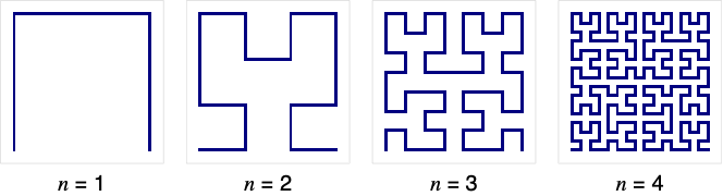
Table[Graphics[HilbertCurve[n]], {n, 5}]Table[RegionMeasure[HilbertCurve[n]], {n, 5}]//RationalizeFindSequenceFunction[%, n]Table[Graphics3D[HilbertCurve[n, 3]], {n, 4}]Table[RegionMeasure[HilbertCurve[n, 3]], {n, 4}]//RationalizeFindSequenceFunction[%, n]DataRangerange is equivalent to using RescalingTransform[{…},range]:
Region[HilbertCurve[3, DataRange -> {{1, 2}, {1, 3}}], Frame -> True]Use RescalingTransform:
box = TransformedRegion[HilbertCurve[3], RescalingTransform[{{0, 2^3 - 1}, {0, 2^3 - 1}}, {{1, 2}, {1, 3}}]];Region[box, Frame -> True]Possible Issues (2)
By default, the coordinates of the Hilbert curve are not in the unit square:
HilbertCurve[2]Using DataRange to generate the Hilbert curve in the unit square:
HilbertCurve[2, DataRange -> {{0, 1}, {0, 1}}]HilbertCurve can be too large to generate:
HilbertCurve[30]Text
Wolfram Research (2017), HilbertCurve, Wolfram Language function, https://reference.wolfram.com/language/ref/HilbertCurve.html.
CMS
Wolfram Language. 2017. "HilbertCurve." Wolfram Language & System Documentation Center. Wolfram Research. https://reference.wolfram.com/language/ref/HilbertCurve.html.
APA
Wolfram Language. (2017). HilbertCurve. Wolfram Language & System Documentation Center. Retrieved from https://reference.wolfram.com/language/ref/HilbertCurve.html