InhomogeneousPoissonPointProcess[μ,d]
represents an inhomogeneous Poisson point process with density function ![]() in
in ![]() .
.


InhomogeneousPoissonPointProcess
InhomogeneousPoissonPointProcess[μ,d]
represents an inhomogeneous Poisson point process with density function ![]() in
in ![]() .
.
Details
- InhomogeneousPoissonPointProcess is also known as a nonstationary Poisson point process or an independent scattering point process.
- Typical uses include modeling varying density that depends only on the location
 , such as varying growth conditions.
 - InhomogeneousPoissonPointProcess generates points in a region according to the specified density function μ with no point interactions.
- With density function μ, the point count in an observation region
 is distributed as PoissonDistribution with mean
  .
. -


- Density function μ can be given as:
-
func a function of vectors geofunc a function of geo locations PointDensityFunction density function from point collections - The number of points
 in disjoint regions
  for a Poisson point process are independent
  , where
  are non-negative integers.
 - A point configuration
 with density function μ in an observation region
  with volume
  has density function
  with respect to PoissonPointProcess[1,d].
 - The Papangelou conditional density
 for adding a point
  to a point configuration
  is
is  for an inhomogeneous Poisson point process with density function μ.
 - The density function
 can be any positive integrable function in
  and d can be any positive integer.
 - InhomogeneousPoissonPointProcess can be used with such functions as RipleyK and RandomPointConfiguration.
Examples
open all close allBasic Examples (4)
Sample from an InhomogeneousPoissonPointProcess:
reg = Disk[];
pts = RandomPointConfiguration[InhomogeneousPoissonPointProcess[Function[{x, y}, 10 * Exp[x + 5y]], 2], reg]Show[RegionPlot[reg], ListPlot[pts]]Sample from an InhomogeneousPoissonPointProcess defined on the surface of the Earth:
reg = Entity["Country", "Japan"]["Polygon"]f = Function[gp, Module[{lat, lon},
{lat, lon} = gp["LatitudeLongitude"];
Quantity[Abs[(lat - lon) / 10 ^ 5], "Kilometers" ^ -2]
]];pts = RandomPointConfiguration[InhomogeneousPoissonPointProcess[f, 2], reg]GeoListPlot[pts]Sample from a nonparametric point density:
pts = SpatialPointData[{{{0.26253893464279254, 0.6772269804041016},
   {0.5740634189787224, 0.8066129928323332}, {0.6812816146974968, 0.685958841359902},
   {-0.1243183062511535, 0.8436689345054196}, {0.4976660640246506, 0.4942748827484774},
   {-0.11 ... rateBoundaries" -> False, "TJunction" -> Automatic, "PropagateMarkers" -> True,
      "ZeroTest" -> Automatic, "Hash" -> 2612179028752913945}], "GeoQ" -> False, "Dimension" -> 2,
"RegionMeasure" -> 1.4784645389892994, "AnnotationsList" -> {}]];λ = SmoothPointDensity[pts]sample = RandomPointConfiguration[InhomogeneousPoissonPointProcess[λ, 2], pts["ObservationRegion"]]ListPlot[{pts["Points"], sample["Points"]}]pts = RandomPoint[Disk[], 100];
density = HistogramPointDensity[pts]Define a point process with the computed point density function and check if it is valid:
proc = InhomogeneousPoissonPointProcess[density, 2];
proc//PointProcessParameterQ
Simulate multiple point configurations:
res = RandomPointConfiguration[proc, Disk[], 2]ListPlot[res]Scope (4)
Simulate several realizations:
pts = RandomPointConfiguration[InhomogeneousPoissonPointProcess[Function[{x, y}, Abs[10 * x + y] * 100], 2], Disk[], 3]pts["PointCountList"]ListPlot[pts, AspectRatio -> 1]Sample from any valid RegionQ, whose RegionEmbeddingDimension is equal to its RegionDimension:
ℛ = ImplicitRegion[x ^ 2 - 2y ^ 2 <= 1, {{x, -3, 3}, {y, -4, 4}}];{RegionQ[ℛ], RegionEmbeddingDimension[ℛ] == RegionDimension[ℛ]}pts = RandomPointConfiguration[InhomogeneousPoissonPointProcess[Function[{x, y}, Exp[x + y]], 2], ℛ]Show[RegionPlot[pts["ObservationRegion"], PlotPoints -> 5], ListPlot[pts]]Gaussian scattering is an example of isotropic inhomogeneous Poisson point process:
proc = InhomogeneousPoissonPointProcess[Function[{x, y}, 3 / 2Exp[14 / 10Norm[{x, y}]]], 2];Simulate the process over a rectangle:
sample = RandomPointConfiguration[proc, Rectangle[{-3, -3}, {3, 3}]]ListPlot[sample]PointCountDistribution is invariant with respect to a rotation about the origin:
region1 = Disk[{1, 0}, 1];dist1 = PointCountDistribution[N[proc, 20], region1]Point count distribution in the rotated region:
region2 = TransformedRegion[region1, RotationTransform[π / 4]]dist2 = PointCountDistribution[N[proc, 20], region2]//QuietThe distributions are the same as identified by equal means:
Mean[dist1] - Mean[dist2]//Chopλ = Function[{x, y},
Piecewise[{{100, (x + 2) ^ 2 + y ^ 2 > 1 && (x - 2) ^ 2 + y ^ 2 > 1}, {1000, (x + 2) ^ 2 + y ^ 2 < 1}}, 0]
];ContourPlot[λ[x, y], {x, -4, 4}, {y, -4, 4}, Contours -> {0, 100, 1000}, ColorFunction -> "TemperatureMap"]proc = InhomogeneousPoissonPointProcess[λ, 2];sample = RandomPointConfiguration[proc, Rectangle[{-4, -4}, {4, 4}]]PointValuePlot[sample]Options (1)
Method (1)
Sample from an InhomogeneousPoissonPointProcess using different methods:
reg = Ellipsoid[{0, 0}, {2, 1.5}];proc = InhomogeneousPoissonPointProcess[Function[{x, y}, 15 * Exp[x + 2 y]], 2];pts1 = RandomPointConfiguration[proc, reg, Method -> "Thinning"]Use the Markov chain Monte Carlo method:
pts2 = RandomPointConfiguration[proc, reg, Method -> "MCMC"]Table[Show[RegionPlot[reg], ListPlot[k], AspectRatio -> Automatic], {k, {pts1, pts2}}]Applications (2)
Point process with density depending on the distance to a line, like a fault line:
λ = Function[{x, y}, 100Exp[-Simplify[RegionDistance[Line[{{-1, -1}, {1, 1}}], {x, y}]^2]]
];Plot3D[λ[x, y], {x, -3, 3}, {y, -3, 3}, MeshFunctions -> {#3&}, Mesh -> 10, Exclusions -> None, ViewPoint -> {0, -3, 3}]proc = InhomogeneousPoissonPointProcess[λ, 2];reg = Rectangle[{-3, -3}, {3, 3}];sample = RandomPointConfiguration[proc, reg]PointValuePlot[sample]Simulate possible point pattern of seeds fallen around a tree:
λ = Function[{x, y}, Piecewise[{{100Exp[-RegionDistance[Disk[], {x, y}]], x ^ 2 + y ^ 2 > 1}}, 0]
];ContourPlot[λ[x, y], {x, -3, 3}, {y, -3, 3}]proc = InhomogeneousPoissonPointProcess[λ, 2];reg = Rectangle[{-3, -3}, {3, 3}];sample = RandomPointConfiguration[proc, reg]PointValuePlot[sample]Properties & Relations (5)
Inhomogeneous Poisson point process with constant density autoevaluates to PoissonPointProcess:
InhomogeneousPoissonPointProcess[λ, 2]The expected number of points in a region for InhomogeneousPoissonPointProcess follows a PoissonDistribution:
proc = InhomogeneousPoissonPointProcess[Function[{x, y}, Sqrt[x ^ 2 + y ^ 2]], 2];Compute the point count distribution over a rectangle:
rec = Rectangle[{0, 0}, {1, 1}];PointCountDistribution[proc, rec]disk = Disk[{0, 0}, r];Assuming[r > 0, PointCountDistribution[proc, disk]]reg = ImplicitRegion[Abs[x] - Abs[y] <= 1, {{x, -3, 3}, {y, -4, 4}}];PointCountDistribution[proc, reg]Compute void probabilities for an inhomogeneous Poisson point process:
proc = InhomogeneousPoissonPointProcess[Function[{x, y}, x ^ 2 + Exp[y]], 2];reg1 = Disk[];PDF[PointCountDistribution[proc, reg1], 0]%//Nreg2 = Rectangle[{-1, -1}, {1, 1}];PDF[PointCountDistribution[proc, reg2], 0]%//Nreg3 = Rectangle[{0, 0}, {2, 2}];PDF[PointCountDistribution[proc, reg3], 0]%//NInhomogeneous Poisson point process is not stationary—the density depends on the location:
proc = InhomogeneousPoissonPointProcess[Function[{x, y}, Exp[x + y]], 2];Point count distribution in a subregion:
subreg1 = Disk[{0, 0}, 1];dist1 = PointCountDistribution[proc, subreg1]Point count distribution in the translated subregion:
subreg2 = Disk[{RandomInteger[], RandomInteger[]}, 1];The region measures are the same:
RegionMeasure[subreg1] == RegionMeasure[subreg2]subreg2The densities as expressed via PointCountDistribution differ:
dist2 = PointCountDistribution[proc, subreg2]dist1 === dist2InhomogeneousPoissonPointProcess with a constant density function is PoissonPointProcess:
proc2D = InhomogeneousPoissonPointProcess[Function[{x, y}, a], 2];The point count distribution in a disk:
disk = Disk[{0, 0}, r];Assuming[r > 0, PointCountDistribution[proc2D, disk]]Point count distribution for a corresponding Poisson point process in the same region:
Assuming[r > 0, PointCountDistribution[PoissonPointProcess[a, 2], disk]]proc3D = InhomogeneousPoissonPointProcess[Function[{x, y, z}, a], 3];ball = Ball[{0, 0, 0}, r];The point count distribution in a ball:
Assuming[r > 0, PointCountDistribution[proc3D, ball]]Point count distribution for a corresponding Poisson point process in the same region:
Assuming[r > 0, PointCountDistribution[PoissonPointProcess[a, 3], ball]]Neat Examples (1)
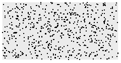
ℛ = [image];𝒫 = InhomogeneousPoissonPointProcess[Function[{x, y}, Exp[-0.02RegionDistance[ℛ][{x, y}]^2]], 2];
sample = RandomPointConfiguration[𝒫, Rectangle[{-50, -20}, {550, 150}]];ListPlot[sample, Frame -> False, Axes -> False]Text
Wolfram Research (2020), InhomogeneousPoissonPointProcess, Wolfram Language function, https://reference.wolfram.com/language/ref/InhomogeneousPoissonPointProcess.html.
CMS
Wolfram Language. 2020. "InhomogeneousPoissonPointProcess." Wolfram Language & System Documentation Center. Wolfram Research. https://reference.wolfram.com/language/ref/InhomogeneousPoissonPointProcess.html.
APA
Wolfram Language. (2020). InhomogeneousPoissonPointProcess. Wolfram Language & System Documentation Center. Retrieved from https://reference.wolfram.com/language/ref/InhomogeneousPoissonPointProcess.html