HistogramPointDensity[pdata]
estimates the histogram point density function ![]() for point data pdata.
for point data pdata.
HistogramPointDensity[pdata,bspec]
estimates the histogram point density function ![]() with histogram bins specified by bspec.
with histogram bins specified by bspec.
HistogramPointDensity[bdata,…,…]
estimates the histogram point density function ![]() for binned data bdata.
for binned data bdata.
HistogramPointDensity[pproc,…,…]
computes the histogram point density function ![]() for the point process pproc.
for the point process pproc.


HistogramPointDensity
HistogramPointDensity[pdata]
estimates the histogram point density function ![]() for point data pdata.
for point data pdata.
HistogramPointDensity[pdata,bspec]
estimates the histogram point density function ![]() with histogram bins specified by bspec.
with histogram bins specified by bspec.
HistogramPointDensity[bdata,…,…]
estimates the histogram point density function ![]() for binned data bdata.
for binned data bdata.
HistogramPointDensity[pproc,…,…]
computes the histogram point density function ![]() for the point process pproc.
for the point process pproc.
Details and Options
- Point density is also known as point intensity.
- HistogramPointDensity gives a function
 that describes how the number of points
  varies per length, area and volume in the observation region
  . The integral over the region is the total number of points
  .
. - HistogramPointDensity is a partition-based estimator of the point density, where the bin specification bspec is used to control the smoothing.
- Histogram point density is typically used to define an inhomogeneous Poisson process or a measure of inhomogeneity.
- HistogramPointDensity returns a PointDensityFunction that can be used to evaluate the density function repeatedly.
- The points pdata can have the following forms:
-
{p1,p2,…} points pi GeoPosition[…],GeoPositionXYZ[…],… geographic points SpatialPointData[…] spatial point collection with observation region {pts,reg} point collection pts and observation region reg - If the observation region reg is not given, a region is automatically computed using RipleyRassonRegion.
- The binned data bdata is assumed to come in the form of SpatialBinnedPointData.
- The point process pproc can have the following forms:
-
proc a point process proc with exact formulas {proc,reg} a point process proc and observation region reg based on simulation - The observation region reg should be a parameter-free, full-dimensional and bounded region as tested by SpatialObservationRegionQ.
- The following geometric and geographic bin specifications bspec can be given:
-
MeshRegion[…] explicit MeshRegion with cells "ObservationMesh" discretization of observation region {reg1,reg2, ...} explicit list of disjoint regions shape geometric shape depending on the dimension {shape,"Count"n} aggregated bins to approximately n bins {shape,"Measure"ν} aggregated bins of approximate measure ν {shape,"Diameter"d} aggregated bins of approximate diameter d - Possible settings for shape include:
-
"Triangle" triangle bins in 2D "Square" square bins in 2D "Hexagon" hexagonal bins in 2D - The geometric bins can also be created by providing bspec coordinate-wise:
-
n use n bins {w} use bins of width w {min,max,w} use bins of width w from min to max {{b1,b2,…}} use bins [b1,b2),[b2,b3),… Automatic determine bin widths automatically "name" use a named binning method fw apply fw to get an explicit bin specification {b1,b2,…} {xspec,yspec,…} give different x, y, etc. specifications - Possible named binning methods include:
-
"FreedmanDiaconis" twice the interquartile range divided by the cube root of sample size "Knuth" balance likelihood and prior probability of a piecewise uniform model "Scott" asymptotically minimize the mean square error "Sturges" compute the number of bins based on the length of data "Wand" one-level recursive approximate Wand binning - All the bins are trimmed to intersect with the observation region.
Examples
open all close allBasic Examples (2)
Create a SpatialPointData:
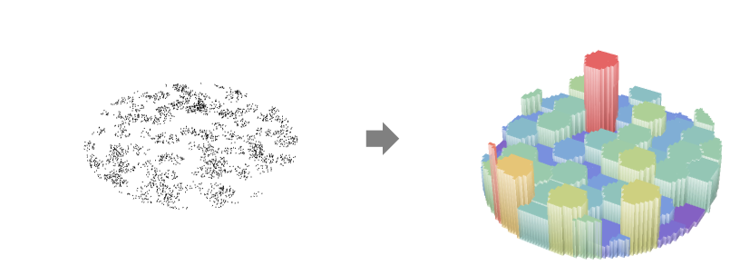
spd = SpatialPointData[RandomReal[1, {300, 2}]];μ = HistogramPointDensity[spd]μ[{.3, .5}]Visualize the density estimation:
DiscretePlot3D[μ[{x, y}], {x, 0, .95, .05}, {y, 0, .95, .05}, ExtentSize -> Full, ColorFunction -> "Rainbow"]Compute histogram point density for a list of geographic points:
data = GeoPosition[{{57.38695860758024, -2.082019036397938}, {64.51592745731402, 45.824927190648225},
  {56.6010212397469, -6.240526809704691}, {51.60678874558969, 57.27710883880354},
  {45.30573867042673, 15.472775964257096}, {47.62531221069711, 33.091 ... 064113254605, 6.294616072872941}, {70.14917097063635, 58.711274282407935},
  {53.9133525034849, 51.235121204775595}, {47.95050112387477, 50.208632516820614},
{45.978247255215074, 0.000929944545532635}, {61.154927383569934, 53.20226357948661}}];μ = HistogramPointDensity[data, "Hexagon"]μ["DensityVisualization"]Scope (5)
Create a homogeneous univariate SpatialPointData:
reg = Rectangle[{0, 0}, {3, 3}];
data = SpatialPointData[RandomPoint[reg, 200], reg]
Compute point density function using different bin shapes:
μ1 = HistogramPointDensity[data, "Triangle"]μ2 = HistogramPointDensity[data, "Hexagon"]Visualize using values at random locations:
sample = RandomPoint[reg, 5 * 10 ^ 3];vals1 = μ1[sample];vals2 = μ2[sample];max = Max[{vals1, vals2}];
colors1 = ColorData["Rainbow"] /@ (vals1 / max);
colors2 = ColorData["Rainbow"] /@ (vals2 / max);ListPlot[MapThread[Style[#1, #2]&, {sample, #}], AspectRatio -> 1, PlotStyle -> PointSize[Medium]]& /@ {colors1, colors2}Histogram point density of clustered data:
data = RandomPointConfiguration[MaternPointProcess[10, 50, .1, 2], Rectangle[]];ListPlot[data, AspectRatio -> Automatic]Compute histogram point density from data:
μ = HistogramPointDensity[data]Show[ContourPlot[μ[{x, y}], {x, 0, 1}, {y, 0, 1}, ContourStyle -> None, ColorFunction -> "SolarColors"], ListPlot[data, PlotStyle -> Black]]Histogram point density for a hardcore process:
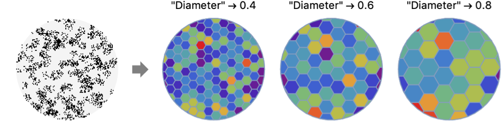
reg = Disk[{0, 0}, 3];
data = RandomPointConfiguration[HardcorePointProcess[10, r = 0.2, 2], reg, Method -> {Automatic, "LengthOfRun" -> 10 ^ 4}];ListPlot[data, AspectRatio -> Automatic]Compute histogram point density from data for various bin diameters:
diams = {r, 2r, 3r};
μ = HistogramPointDensity[data, {"Square", "Diameter" -> #}]& /@ diams;Table[Show[ContourPlot[μ[[k]][{x, y}], {x, -3, 3}, {y, -3, 3}, ContourStyle -> None, ColorFunction -> "PearlColors", PlotLabel -> Row[{"bandwidth = ", diams[[k]]}]], ListPlot[data, PlotStyle -> Black]], {k, 3}]Compare bin shape specifications:
sp = SpatialPointData[RandomReal[1, {50, 2}], Rectangle[]];Define a mesh region and polygon composite region:
mesh = [image];polygonlist = MeshPrimitives[mesh, 2];pfs = Table[HistogramPointDensity[sp, type], {type, {"MeshRegion", "AggregatedMeshRegion", "Hexagon", "Square", "Triangle", mesh, polygonlist}}];types = {"MeshRegion", "AggregatedMeshRegion", "Hexagon", "Square", "Triangle", "mesh", "polygonlist"};MapThread[Show[Labeled[#1["DensityVisualization"], #2], ImageSize -> 110]&, {pfs, types}]Allowed bin specifications on the surface of the Earth:
pts = SpatialPointData@RandomGeoPosition[Entity["Country", "Italy"], 100];GeoListPlot[pts["Points"]]pfs = Table[HistogramPointDensity[pts, type], {type, {"MeshRegion", "AggregatedMeshRegion", "Hexagon", "Square", "Triangle"}}];GraphicsRow@Table[Show[pf["DensityVisualization"], ImageSize -> 100], {pf, pfs}]//QuietApplications (1)
Get the data of rat sightings in New York City:
tab = Tabular[ResourceData["NYC Rat Sightings"]]List column keys to find locations column:
ColumnKeys[tab]Extract geo locations, delete missing and create SpatialPointData:
pts = DeleteMissing[Normal[tab[All, "GeoLocation"]]];locs = SpatialPointData[pts]Compute histogram point density:
density = HistogramPointDensity[locs]Visualize the areas of prevalence of rat sightings in NYC on a sample of the locations:
pos = RandomSample[pts, 3000];
vals = density[pos];PointValuePlot[pos -> vals, ColorFunction -> "Rainbow", PlotStyle -> PointSize[Small], GeoBackground -> "VectorMonochrome"]Properties & Relations (1)
HistogramPointDensity is related to Histogram with bin height specification "Intensity":
data1 = RandomPointConfiguration[PoissonPointProcess[100, 1], Interval[{-1, 1}]];Specifying bin width in computation of histogram point density:
μ1 = HistogramPointDensity[data1, {.1}]Compare the density function to the intensity Histogram with the same bin width:
Show[Histogram[data1, {.1}, "Intensity"], Plot[μ1[{x}], {x, -1, 1}]]data2 = RandomPointConfiguration[PoissonPointProcess[100, 2], Rectangle[]];ListPlot[data2]Compute histogram point intensity:
μ2 = HistogramPointDensity[data2, {.1}]Compare plot of the density function with the Histogram3D of the data:
μplot = DiscretePlot3D[μ2[{x, y}], {x, 0, 1, .1}, {y, 0, 1, .1}, ExtentSize -> Right, ColorFunction -> "Rainbow", PlotRange -> {{0, 1}, {0, 1}, All}];h = Histogram3D[data2, {.1}, "Intensity", ColorFunction -> (ColorData["Rainbow"][Rescale[#, {0, 1}, {0.25, 1}]]&)];{μplot, h}Text
Wolfram Research (2020), HistogramPointDensity, Wolfram Language function, https://reference.wolfram.com/language/ref/HistogramPointDensity.html.
CMS
Wolfram Language. 2020. "HistogramPointDensity." Wolfram Language & System Documentation Center. Wolfram Research. https://reference.wolfram.com/language/ref/HistogramPointDensity.html.
APA
Wolfram Language. (2020). HistogramPointDensity. Wolfram Language & System Documentation Center. Retrieved from https://reference.wolfram.com/language/ref/HistogramPointDensity.html