

KochCurve
Details and Options
- KochCurve is also known as Koch snowflake.
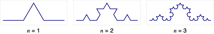
- KochCurve[n] is generated from the unit interval by repeatedly removing the middle third of the subsequent cells and replacing it with a triangle. »
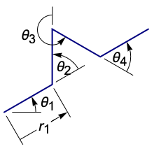
- KochCurve[n] is equivalent to KochCurve[n,{0,60 °,-120 °,60 °}].
- KochCurve takes a DataRange option that can be used to specify the range the coordinates should be assumed to occupy.
Examples
open all close allBasic Examples (2)
Graphics[KochCurve[2]]Lengths of the approximations to the Koch mesh:
Table[ArcLength[KochCurve[n]], {n, 5}]//RationalizeFindSequenceFunction[%, n]The first four iterations of the Koch snowflake:
Table[Graphics[GeometricTransformation[KochCurve[i], {RotationTransform[Pi, {1 / 2, 0}], RotationTransform[-Pi / 3, {1, 0}], RotationTransform[Pi / 3, {0, 0}]}]], {i, 4}]Scope (7)
Curve Specification (3)
Graphics[KochCurve[2]]The n![]() approximation of the Koch curve:
approximation of the Koch curve:
Table[Graphics[KochCurve[n]], {n, 1, 4}]Specify the length of the relative angles:
Graphics@KochCurve[2, {{1, 0}, {1, 90°}, {1, -90°}, {2, -90°}, {1, 90°}, {1, 90°}, {1, -90°}}]Curve Styling (4)
Koch curves with different thicknesses:
Table[Graphics[{Thickness[i], KochCurve[3]}], {i, {Medium, Large}}]Table[Graphics[{Thickness[i], KochCurve[2]}], {i, {.005, .05, .1}}]Thickness in printer's points:
Table[Graphics[{AbsoluteThickness[i], KochCurve[2]}], {i, {1, 5, 10}}]Table[Graphics[{Dashing[i], KochCurve[3]}], {i, {Tiny, Small, Medium, Large}}]Table[Graphics[{d, KochCurve[3]}], {d, {Dotted, Dashed, DotDashed}}]Table[Graphics[{c, KochCurve[3]}], {c, {Red, Green, Blue, Yellow}}]Options (1)
DataRange (1)
DataRange allows you to specify the range of mesh coordinates to generate:
KochCurve[1]KochCurve[1, DataRange -> {{-1, 1}, {-1, 1}}]Applications (4)
KochCurve is generated by repeatedly removing the middle third of the cells and replacing it with a triangle:
Column[Table[Graphics[KochCurve[n]], {n, 1, 3}]]Graphics[KochCurve[3, {0, 85°, -85°, -85°, 85°}]]Graphics[KochCurve[3, {0, 90°, -90°, -90°, 90°}]]Graphics[KochCurve[3, {{1, 0}, {1, 90°}, {1, -90°}, {2, -90°}, {1, 90°}, {1, 90°}, {1, -90°}}]]Properties & Relations (3)
KochCurve consists of lines:
KochCurve[1]AnglePath can be used to generate the first iteration of the Koch curve:
path = {{1, 0}, {1, 90°}, {1, -90°}, {1, -90°}, {1, 0°}, {1, 90°}, {1, 90°}, {1, -90°}};{Graphics[KochCurve[1, path]], Graphics[Line[AnglePath[path]]]}DataRange -> range is equivalent to using RescalingTransform[{...},range]:
Region[KochCurve[2, DataRange -> {{1, 2}, {1, 3}}], Frame -> True]Use RescalingTransform:
box = TransformedRegion[mr = KochCurve[2], RescalingTransform[RegionBounds[mr], {{1, 2}, {1, 3}}]];Region[box, Frame -> True]Text
Wolfram Research (2017), KochCurve, Wolfram Language function, https://reference.wolfram.com/language/ref/KochCurve.html.
CMS
Wolfram Language. 2017. "KochCurve." Wolfram Language & System Documentation Center. Wolfram Research. https://reference.wolfram.com/language/ref/KochCurve.html.
APA
Wolfram Language. (2017). KochCurve. Wolfram Language & System Documentation Center. Retrieved from https://reference.wolfram.com/language/ref/KochCurve.html