Wolfram Language & System Documentation Center

ObservableDecomposition

yields the observable subsystem of the system sys.

ObservableDecomposition[sys,{z₁,…}]

specifies the new coordinates z_i.

Details and Options

ObservableDecomposition gives {p,osys}, where p is the transformation and osys is the observable subsystem.
The system sys can be a standard or descriptor StateSpaceModel or AffineStateSpaceModel.
The observable subsystem is given by StateSpaceTransform[sys,p].
ObservableDecomposition accepts a Method option. The following settings can be specified:
Automatic automatically choose the method

"Matrix" use the observability matrix

"Distribution" use the observability distribution

Examples

open all close all

Basic Examples (1)

Find the observable subsystem and its transformation:

Wolfram Language code:

ObservableDecomposition[StateSpaceModel[{{{Subscript[a, 1], 0, 0}, {0, Subscript[a, 2], 0}, 
   {0, 0, Subscript[a, 3]}}, {{Subscript[b, 1]}, 
   {Subscript[b, 2]}, {Subscript[b, 3]}}, 
  {{Subscript[c, 1], 0, Subscript[c, 3]}}, 
  {{Subscript[d, 11]}}}, SamplingPeriod -> None, SystemsModelLabels -> None]]

Scope (4)

The observable subsystem of an observable system is the complete system:

Wolfram Language code:

ssm = StateSpaceModel[{{{0, 0, -2}, {1, 0, -3}, {0, 1, -1}}, {{3}, {-2}, {1}}, {{0, 0, 1}}, {{0}}}, 
 SamplingPeriod -> None, SystemsModelLabels -> None];
ObservableDecomposition[ssm]

The observable subsystem of a partially observable continuous-time system:

Wolfram Language code:

ssm = StateSpaceModel[{{{3, 6, 4}, {9, 6, 10}, {-7, -7, -9}}, {{1/3, 2/3}, {2/3, 1/3}, {-1/6, 1/3}}, 
  {{1, 2, 3}, {3, 3, 6}}, {{0, 0}, {0, 0}}}, SamplingPeriod -> None, SystemsModelLabels -> None];

Wolfram Language code: MatrixForm /@ ObservableDecomposition[N@ssm]

The observable subsystem of a descriptor system:

Wolfram Language code:

ObservableDecomposition[StateSpaceModel[{{{Subscript[a, 1], 0, 0}, {0, Subscript[a, 2], 0}, 
   {0, 0, Subscript[a, 3]}}, {{0, 0}, {Subscript[b, 1], 0}, 
   {0, Subscript[b, 2]}}, {{0, Subscript[c, 1], 0}, 
   {0, 0, Subscript[c, 3]}}, 
  {{Subscript[d, 11], Subscript[d, 12]}, 
   {Subscript[d, 21], Subscript[d, 22]}}, 
  {{Subscript[e, 1], 0, 0}, {0, Subscript[e, 2], 0}, {0, 0, 0}}}, 
 SamplingPeriod -> None, SystemsModelLabels -> None]]

The observable subsystem of an affine system:

Wolfram Language code:

ObservableDecomposition[AffineStateSpaceModel[{{-Subscript[x, 2], Subscript[x, 1]*
    Subscript[x, 2], Subscript[x, 3]}, 
  {{1 + Subscript[x, 2]}, {0}, {0}}, {Subscript[x, 1]}, {{0}}}, 
 {Subscript[x, 1], Subscript[x, 2], Subscript[x, 3]}, 
 {Subscript[, 1]}, {Automatic}, Automatic, SamplingPeriod -> None]]

Specify the new variables:

Wolfram Language code:

ObservableDecomposition[AffineStateSpaceModel[{{-Subscript[x, 2], Subscript[x, 1]*
    Subscript[x, 2], Subscript[x, 3]}, 
  {{1 + Subscript[x, 2]}, {0}, {0}}, {Subscript[x, 1]}, {{0}}}, 
 {Subscript[x, 1], Subscript[x, 2], Subscript[x, 3]}, 
 {Subscript[, 1]}, {Automatic}, Automatic, SamplingPeriod -> None], {Subscript[z, 1], Subscript[z, 2], Subscript[z, 3]}]

Applications (7)

Linear Systems (4)

Construct the Kalman observable decomposition:

Wolfram Language code:

ssm = StateSpaceModel[{{{Subscript[a, 1], 0, 0}, {0, Subscript[a, 2], 0}, 
   {0, 0, Subscript[a, 3]}}, {{0, 0}, {Subscript[b, 1], 0}, 
   {0, Subscript[b, 2]}}, {{Subscript[c, 1], 0, 0}, 
   {0, 0, Subscript[c, 3]}}, 
  {{Subscript[d, 11], Subscript[d, 12]}, 
   {Subscript[d, 21], Subscript[d, 22]}}}, SamplingPeriod -> None, 
 SystemsModelLabels -> None];

ObservableDecomposition picks out the observable subsystem only:

Wolfram Language code: {p, ossm} = ObservableDecomposition[ssm];

Wolfram Language code: ossm

Kalman observable decomposition puts the observable subsystem first and keeps the rest:

Wolfram Language code:

po = NullSpace[p]; (* Orthogonal space *)
StateSpaceTransform[ssm, ArrayFlatten[{{p, po}}]]

Compute the dimension of the observable subspace:

Wolfram Language code:

{p, ossm} = ObservableDecomposition[StateSpaceModel[{{{Subscript[a, 1], 0, 0}, {0, Subscript[a, 2], 0}, 
   {0, 0, Subscript[a, 3]}}, {{0, 0}, {Subscript[b, 1], 0}, 
   {0, Subscript[b, 2]}}, {{Subscript[c, 1], 0, 0}, 
   {0, 0, Subscript[c, 3]}}, 
  {{Subscript[d, 11], Subscript[d, 12]}, 
   {Subscript[d, 21], Subscript[d, 22]}}}, SamplingPeriod -> None, 
 SystemsModelLabels -> None]];

The observable subspace is the range of p, i.e. the column dimension:

Wolfram Language code: Dimensions[p]//Last

Find the observable subspace for the system below and show what state trajectories you can tell apart from observing the output only:

Wolfram Language code:

ssm = StateSpaceModel[{{{-6, -2, -3}, {3, -1, 3}, {2, 2, -1}}, {{1}, {0}, {-2}}, {{0, 1, -1}}, {{0}}}, 
 SamplingPeriod -> None, SystemsModelLabels -> None];

The system is unobservable, so only a subspace is observable from output:

Wolfram Language code: ObservableModelQ[ssm]

The range of the transformation p gives the observable subspace:

Wolfram Language code: {p, osys} = ObservableDecomposition[ssm];

Wolfram Language code: ospace = ParametricPlot3D[p.{u, v}, {u, -1, 1}, {v, -1, 1}, Mesh -> None, PlotStyle -> Opacity[0.7]]

Simulate trajectories whose initial value projects to a single point on the observable subspace:

Wolfram Language code:

w = First@NullSpace[p];
x0 = Table[p.{0.5, 0.5} + λ w, {λ, -0.4, 0.4, 0.2}];
sr = Table[StateResponse[{ssm, x}, Sin[2t], {t, 0, 10}], {x, x0}];

Wolfram Language code:

Show[ParametricPlot3D[Evaluate[sr], {t, 0, 10}], ospace, ParametricPlot3D[Evaluate[p.{0.5, 0.5} + λ w], {λ, -0.5, 0.5}]]

From observing the output, all these trajectories look identical:

Wolfram Language code: or = Table[OutputResponse[{ssm, x}, Sin[2t], {t, 0, 10}], {x, x0}];

Wolfram Language code: Plot[or, {t, 0, 10}]

Determine states that can be estimated using available measurements and design an estimator:

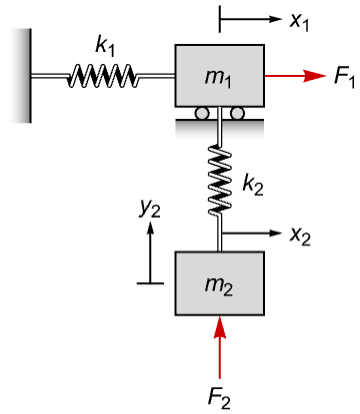
Only the position of mass is measured, and so the system is not completely observable:

Wolfram Language code: pars = {Subscript[k, 1] -> 75, Subscript[k, 2] -> 100, Subscript[m, 1] -> 1, Subscript[m, 2] -> 0.5};

Wolfram Language code:

ssm  = StateSpaceModel[{{{0, 1, 0, 0, 0, 0}, 
   {-(Subscript[k, 1] + Subscript[k, 2])/Subscript[m, 1], 0, 
    Subscript[k, 2]/Subscript[m, 1], 0, 0, 0}, {0, 0, 0, 1, 0, 0}, 
   {Subscript[k, 2]/Subscript[m, 2], 0, 
    -Subscript[k, 2]/Subscript[m, 2], 0, 0, 0}, {0, 0, 0, 0, 0, 1}, 
   {0, 0, 0, 0, -Subscript[k, 2]/Subscript[m, 2], 0}}, 
  {{0, 0}, {Subscript[m, 1]^(-1), 0}, {0, 0}, {0, 0}, {0, 0}, 
   {0, Subscript[m, 2]^(-1)}}, {{1, 0, 0, 0, 0, 0}}, {{0, 0}}}, 
 SamplingPeriod -> None, SystemsModelLabels -> 
  {None, None, {Subscript[x, 1], Subscript[v, 1], 
    Subscript[x, 2], Subscript[v, 2*x], 
    Subscript[y, 2], Subscript[v, 2*y]}}]  /. pars;

Wolfram Language code: ObservableModelQ[ssm]

The states associated with zero rows in the transformation matrix cannot be observed:

Wolfram Language code: {p, osys} = ObservableDecomposition[ssm];

Wolfram Language code: Position[p, {_ ? PossibleZeroQ..}]

An estimator can be designed to estimate any combination of the first four states:

Wolfram Language code: ℓ = EstimatorGains[osys, {-1, -2, -3 + I, -3 - I}]

An estimator that estimates :

Wolfram Language code: StateOutputEstimator[osys, ℓ];

Wolfram Language code: est = SystemsModelSeriesConnect[%, TransferFunctionModel[{PadRight[p[[3]], 5]}]]

Compute the response of for a set of input signals and initial conditions:

Wolfram Language code:

inps = {UnitStep[t] - UnitStep[t - 2], UnitStep[t - 1] - UnitStep[t - 3]};
ics = {0.01, 0, 0.1, 0, 0.05, 0};

Wolfram Language code:

x2 = StateResponse[{ssm, ics}, inps, {t, 0, 8}][[3]];
Plot[x2, {t, 0, 8}]

The estimated state trajectories:

Wolfram Language code: x2e = OutputResponse[est, Join[inps, OutputResponse[{ssm, ics}, inps, {t, 0, 8}]], {t, 0, 8}];

Wolfram Language code: Plot[{x2, x2e}, {t, 0, 8}, PlotLegends -> {"actual", "estimated"}, PlotRange -> All]

Affine Systems (3)

Construct the triangular observability decomposition:

Wolfram Language code:

assm = AffineStateSpaceModel[{{Subscript[x, 1], -Subscript[x, 1] + 
    Subscript[x, 2] + Subscript[x, 1]*Subscript[x, 2], 
   -Subscript[x, 1] - Subscript[x, 3]}, 
  {{0}, {1}, {1 + Subscript[x, 1]}}, {Subscript[x, 2]}, {{0}}}, 
 {Subscript[x, 1], Subscript[x, 2], Subscript[x, 3]}, 
 Automatic, {Automatic}, Automatic, SamplingPeriod -> None];

ObservableDecomposition picks out the observable subsystem only:

Wolfram Language code: {{p1, p2}, osys} = ObservableDecomposition[assm];

Wolfram Language code: osys

Triangular observability decomposition puts the observable subsystem first and keeps the rest:

Wolfram Language code: StateSpaceTransform[assm, {p1, Flatten[p2]}]

Compute the dimension of the observable subspace:

Wolfram Language code:

assm = AffineStateSpaceModel[{{E^Subscript[x, 2]*Subscript[x, 2] + 
    Subscript[x, 1]*Subscript[x, 3], Subscript[x, 3], 
   (-Subscript[x, 2])*Subscript[x, 3] + Subscript[x, 4], 
   (-Subscript[x, 2]^2)*Subscript[x, 3] + 
    Subscript[x, 3]^2 + Subscript[x, 2]*Subscript[x, 4]}, 
  {{Subscript[x, 1]}, {1}, {0}, {Subscript[x, 3]}}, 
  {Subscript[x, 3]}, {{0}}}, {Subscript[x, 1], 
  Subscript[x, 2], Subscript[x, 3], Subscript[x, 4]}, 
 Automatic, {Automatic}, Automatic, SamplingPeriod -> None];

Wolfram Language code: ObservableModelQ[assm]

The dimension can be obtained from the inverse transformation :

Wolfram Language code: {{Subscript[p, 1], Subscript[p, 2]}, ossm} = ObservableDecomposition[assm];

Wolfram Language code: ossm

Wolfram Language code: Length[First[Subscript[p, 2]]]

Find the subspaces whose outputs are indistinguishable:

Wolfram Language code:

asys = AffineStateSpaceModel[{{E^Subscript[x, 2]*Subscript[x, 2] + 
    Subscript[x, 1]*Subscript[x, 3], Subscript[x, 3], 
   (-Subscript[x, 2])*Subscript[x, 3] + Subscript[x, 4], 
   (-Subscript[x, 2]^2)*Subscript[x, 3] + 
    Subscript[x, 3]^2 + Subscript[x, 2]*Subscript[x, 4]}, 
  {{Subscript[x, 1]}, {1}, {0}, {Subscript[x, 3]}}, 
  {Subscript[x, 3]}, {{0}}}, {Subscript[x, 1], 
  Subscript[x, 2], Subscript[x, 3], Subscript[x, 4]}, 
 Automatic, {Automatic}, Automatic, SamplingPeriod -> None];

The system is unobservable, so only a subspace is observable from output:

Wolfram Language code: ObservableModelQ[asys]

The indistinguishable subspace:

Wolfram Language code: {{Subscript[p, 1], {Subscript[p, 21], Subscript[p, 22]}}, osys} = ObservableDecomposition[asys];

Wolfram Language code:

isubspace[{x1_, x2_, x3_, x4_}] := Last /@ Subscript[p, 21] /. {Subscript[x, 1] -> x1, Subscript[x, 2] -> x2, Subscript[x, 3] -> x3, Subscript[x, 4] -> x4}

Wolfram Language code: isubspace[{Subscript[x, 1], Subscript[x, 2], Subscript[x, 3], Subscript[x, 4]}]

Two points on the subspace:

Wolfram Language code:

Subscript[pt, 1] = {1, 3, 1, 2};
Subscript[pt, 2] = {1, 1, 1, 0};

Wolfram Language code: isubspace /@ {Subscript[pt, 1], Subscript[pt, 2]}

The trajectories of the outputs from the two points are the same:

Wolfram Language code: Table[OutputResponse[{asys, pt}, UnitStep[t], {t, 0, 1}], {pt, {Subscript[pt, 1], Subscript[pt, 2]}}];

Wolfram Language code: Table[Plot[or, {t, 0, 1}], {or, Flatten[%, 1]}]

Properties & Relations (2)

The transformation matrix p selects the observable subsystem using StateSpaceTransform:

Wolfram Language code:

ssm = StateSpaceModel[{{{Subscript[a, 1], 0, 0}, {0, Subscript[a, 2], 0}, 
   {0, 0, Subscript[a, 3]}}, {{0, 0}, {Subscript[b, 1], 0}, 
   {0, Subscript[b, 2]}}, {{Subscript[c, 1], 0, 0}, 
   {0, 0, Subscript[c, 3]}}, 
  {{Subscript[d, 11], Subscript[d, 12]}, 
   {Subscript[d, 21], Subscript[d, 22]}}}, SamplingPeriod -> None, 
 SystemsModelLabels -> None];

Wolfram Language code:

{p, osys} = ObservableDecomposition[ssm];
tsys = StateSpaceTransform[ssm, {p, p}];

Wolfram Language code: {osys, tsys}

For affine systems, the transformation rules select the observable subsystem:

Wolfram Language code:

assm = AffineStateSpaceModel[{{-Subscript[x, 4], 0, -Subscript[x, 1], 
   Subscript[x, 2]}, {{1}, {0}, {1 + Subscript[x, 2]}, {0}}, 
  {Subscript[x, 1], Subscript[x, 2]}, {{0}, {0}}}, 
 {Subscript[x, 1], Subscript[x, 2], Subscript[x, 3], 
  Subscript[x, 4]}, {Subscript[, 1]}, {Automatic, Automatic}, Automatic, 
 SamplingPeriod -> None];

Wolfram Language code:

{p, osys} = ObservableDecomposition[assm];
tsys = StateSpaceTransform[assm, p];

Wolfram Language code: {osys, tsys}

Top

More Learning

Tech Support

Wolfram Solutions

Wolfram Solutions For Education

Get Started

Grow Your Skills

Work with Us

Educational Programs for Adults

Educational Programs for Youth

Read

ObservableDecomposition

Details and Options

Examples

Basic Examples (1)

Scope (4)

Applications (7)

Linear Systems (4)

Affine Systems (3)

Properties & Relations (2)

Text

CMS

APA

BibTeX

BibLaTeX

	Automatic	automatically choose the method
	"Matrix"	use the observability matrix
	"Distribution"	use the observability distribution

ObservableDecomposition

Details and Options

Examples

Basic Examples (1)

Scope (4)

Applications (7)

Linear Systems (4)

Affine Systems (3)

Properties & Relations (2)

See Also

Related Guides

History

Text

CMS

APA

BibTeX

BibLaTeX