

PolynomialModel
represents a polynomial function with unknown degree.
represents a polynomial function of a given degree n in the input variables.
PolynomialModel[n,vars]
uses an explicit variable specification vars.
PolynomialModel[n,pars,vars]
uses the provided coefficients pars.
Details
- PolynomialModel represents a polynomial in the given variables in a format suitable for symbolic or numerical evaluation and fitting.
- Polynomials are often used to fit smooth nonlinear phenomena such as sensor calibration curves, braking distance with speed, material stress–strain responses and gradual environmental and economic trends over a limited range.
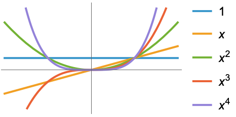
- The univariate polynomial of degree n is given by
![sum _(i=0)^(n)TemplateBox[{i}, CTraditional] x^i](Files/PolynomialModel.en/2.png "sum _(i=0)^(n)TemplateBox[{i}, CTraditional] x^i") .
. - The multivariate polynomial of total degree n is given by
![sum_(i=0)^nsum_(j_1+...+j_k⩵i) c_(j_1,...,j_k)TemplateBox[{{x, _, 1}, {j, _, 1}}, Superscript] TemplateBox[{{..., , {x, _, k}}, {j, _, k}}, Superscript]](Files/PolynomialModel.en/3.png "sum_(i=0)^nsum_(j_1+...+j_k⩵i) c_(j_1,...,j_k)TemplateBox[{{x, _, 1}, {j, _, 1}}, Superscript] TemplateBox[{{..., , {x, _, k}}, {j, _, k}}, Superscript]") .
. - Individual monomials are sorted successively by total degree, max degree and finally, variable order.
- When used in ModelFit, each monomial is used as an independent basis element.
- The current model representation can be expanded using PolynomialModel[…][{x1,…}].
- The following hyperparameters may be specified for this model:
-
"Degree" Automatic polynomial degree - Possible settings for degree include:
-
n degree n UpTo[n] all degrees up to and including n n;;m all degrees between n and m inclusive n;;m;;s all degrees between n and m in steps of s - A limited subset of models may be expressed as PolynomialModel[UpTo[n]].
- When not specified, variables will automatically be enumerated using x[i].
- Valid variable specifications vars include:
-
n the number of variables symb a symbolic representation of a single variable {symb1,…} a list of symbolic variables - When not specified, parameters will automatically be enumerated using C[i].
- Valid parameter pars specifications in the form {par1,…} include:
-
val a fixed parameter value val par a symbolic parameter name par parval a symbolic name par set to a fixed value val - Model properties can be extracted using Information[PowerModel[…],prop].
- Valid basic properties include:
-
"BaseType" model base type "Name" model name "ShortName" short identifier to use as label "InputType" supported input types "OutputType" supported output types - Valid data-related properties include:
-
"ColumnNames" names of the input features "ColumnVariableMap" map between column names and model variables "InputSize" dimensionality of the input "OutputSize" dimensionality of the output "Trainable" whether the model is fully specified and can be trained "Trained" whether the model can be evaluated numerically "VariableColumnMap" map between model variables and column names "Variables" name of the model variables - Best model-related properties include:
-
"Expression" model expression "Function" model as a pure function "SymbolicExpression" model expression with symbolic parameters "TabularFunction" pure function suitable to work on a tabular row - Parameter-related properties include:
-
"ParameterAssociation" association of parameter names and values "ParameterCount" the number of parameters "ParameterInitialValues" initial values for the fit "ParameterNames" parameter names "ParameterRules" list of rules with parameter names and values "Parameters" parameter values if present; names otherwise "ParameterValues" parameter values "Constraints" parameter constraints - Hyperparameter-related properties include:
-
"HyperparameterDefaultDomain" default hyperparameter search domain "HyperparameterDomain" specified hyperparameter search domain "Hyperparameters" hyperparameter values
Hyperparameters
Variables
Parameters
Properties
Examples
open all close allBasic Examples (3)
Specify a quadratic polynomial model:
PolynomialModel[2]Use an explicit input size and custom names for the symbolic parameters:
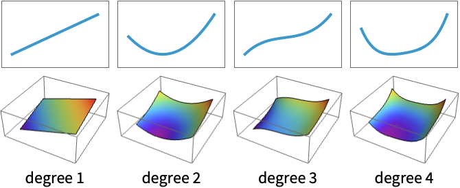
PolynomialModel[2, {a, b, c}, 1]Plot over a variety of degrees using constant parameters:
Plot[{PolynomialModel[1, {1, 1}, 1][x], PolynomialModel[2, {1, 1, 1 }, 1][x], PolynomialModel[3, {1, 1, 1, 1}, 1][x]}, {x, -2, 2}]Scope (24)
Hyperparameters (2)
Degree (2)
Specify the degree of the model:
PolynomialModel[2][x]Specify a family of models with the maximum given degree:
model = PolynomialModel[UpTo[4]]Use ModelFit to find the best polynomial model up to this maximum degree:
ModelFit[1 + Range[10] ^ 2, model]Variables (2)
Specify a PolynomialModel by degree alone:
PolynomialModel[2]The number of variables is inferred from the arguments:
PolynomialModel[2][{x}]
PolynomialModel[2][{x, y, z}]
ModelFit will assume the number of variables is one less than the number of data points:
ModelFit[{{1, 9, 55}, {1, 1, 7}, {1, 4, 25}, {8, 9, 118}, {8, 10, 124}, {8, 5, 94}}, PolynomialModel[2]]Specify the number of variables:
PolynomialModel[2, 2]Give the variables a custom symbolic representation:
PolynomialModel[2, {var1, var2}]These names are overwritten when the model is evaluated symbolically:
PolynomialModel[2, {var1, var2}][{a, b}]Parameters (4)
Parameter names are assigned automatically:
PolynomialModel[2, 1]Specify custom parameter names:
PolynomialModel[2, {a, b, c}, 1]Set a parameter to a specific value:
PolynomialModel[2, {42, b, c}, 1]Specify both parameter names and values:
PolynomialModel[2, {a -> 1, b, c}, 1]Evaluation (5)
Symbolically evaluate a single-variable model:
PolynomialModel[2, 1][x]Symbolically evaluate a two-variable model:
PolynomialModel[2, 2][{x, y}]The number of variables is automatically inferred if not specified:
PolynomialModel[2][x]PolynomialModel[2][{x, y}]Evaluate the model on multiple symbolic variables:
PolynomialModel[2, 2][{{x, y}, {a, b}}]Evaluate the model on a list of points:
PolynomialModel[2, 1][{1, 2, 3}]Information (5)
View general information about a model:
Information[PolynomialModel[2]]Some information is only available when variables or parameters are fully specified:
Information[PolynomialModel[2, x]]Information[PolynomialModel[2, {a, b, c}, {x}], "Variables"]Information[PolynomialModel[2, {a, b, c}, x], {"Variables", "Parameters"}]Get information about the default model values:
Information[PolynomialModel[2, 1], {"Variables", "Parameters"}]Fitting (6)
Fit a polynomial model of the specified degree:
ModelFit[{...}, PolynomialModel[3]]ModelFit[{...}, PolynomialModel[UpTo[5]]]Automatically detect the degree:
ModelFit[{...}, PolynomialModel[]]View the report to compare the fits:
ModelFit[{...}, PolynomialModel[], "Report"]Numerical parameter values are considered fixed during fitting:
ModelFit[{...}, PolynomialModel[1, {1, b}, 1]]Fixing all the parameters will result in a model equivalent to the input:
Information[ModelFit[{...}, PolynomialModel[1, {1, 2}, 1]], "ParameterValues"]Compare the performance of a previously trained model with one trained on the actual data:
report = ModelFit[{...}, {PolynomialModel[2, {1, 2, 3}, 1], PolynomialModel[1]}, "Report"]Extract the parameters for both models:
report["ParameterValues" -> All]Applications (11)
Basic Applications (6)
Fit the area of a rectangle to its width and height:
ModelFit[Tabular[Association["RawSchema" -> Association["ColumnProperties" ->
     Association["Width" -> Association["ElementType" -> "Integer64"],
      "Height" -> Association["ElementType" -> "Integer64"],
      "Volume" -> Association["ElementType" -> "Integer64"]], "KeyColumns" -> None,
    "Backend" -> "WolframKernel"], "Options" -> {},
  "BackendData" -> Association["ColumnData" -> DataStructure["ColumnTable",
      {{TabularColumn[Association["Data" -> {{5, 2, 1, 1, 10, 2, 5, 5, 10, 5}, {}, None},
          "ElementType" -> "Integer64"]], TabularColumn[Association[
          "Data" -> {{1, 1, 10, 5, 10, 5, 10, 2, 2, 5}, {}, None}, "ElementType" -> "Integer64"]],
        TabularColumn[Association["Data" -> {{5, 2, 10, 5, 100, 10, 50, 10, 20, 25}, {}, None},
          "ElementType" -> "Integer64"]]}}]]]], PolynomialModel[]]
Fit the volume of water in a cuboid to its dimensions:
ModelFit[Tabular[Association["RawSchema" -> Association["ColumnProperties" ->
     Association["Width" -> Association["ElementType" -> "Integer64"],
      "Height" -> Association["ElementType" -> "Integer64"],
      "Length" -> Association["ElementType" -> "Integer64"],
      "Volume" -> Association["ElementType" -> "Integer64"]], "KeyColumns" -> None,
    "Backend" -> "WolframKernel"], "Options" -> {},
  "BackendData" -> Association["ColumnData" -> DataStructure["ColumnTable",
      {{TabularColumn[Association["Data" -> {{2, 2, 50, 15, 5, 5, 25, 50, 1, 5, 5, 15, 25, 25, 20,
             25, 25, 20, 25, 2}, {}, None}, "ElementType" -> "Integer64"]],
        TabularColumn[Association["Data" -> {{15, 50, 20, 10, 5, 1, 20, 5, 20, 10, 20, 5, 1, 10,
             20, 20, 5, 20, 2, 15}, {}, None}, "ElementType" -> "Integer64"]],
        TabularColumn[Association["Data" -> {{25, 50, 50, 20, 20, 5, 15, 50, 2, 15, 1, 20, 1, 15,
             2, 1, 50, 20, 15, 5}, {}, None}, "ElementType" -> "Integer64"]],
        TabularColumn[Association["Data" -> {{750, 5000, 50000, 3000, 500, 25, 7500, 12500, 40,
             750, 100, 1500, 25, 3750, 800, 500, 6250, 8000, 750, 150}, {}, None},
          "ElementType" -> "Integer64"]]}}]]]], PolynomialModel[]]
Fit the area of a disc to its radius:
ModelFit[Tabular[Association["RawSchema" -> Association["ColumnProperties" ->
     Association["Radius" -> Association["ElementType" -> "Integer64"],
      "Area" -> Association["ElementType" -> "Real64"]], "KeyColumns" -> None,
    "Backend" -> "WolframKernel"], "Options" -> {},
  "BackendData" -> Association["ColumnData" -> DataStructure["ColumnTable",
      {{TabularColumn[Association["Data" -> {{1, 2, 5, 10, 15, 20, 25, 50}, {}, None},
          "ElementType" -> "Integer64"]], TabularColumn[Association[
          "Data" -> {{3.141592653589793, 12.566370614359172, 78.53981633974483, 314.1592653589793,
             706.8583470577034, 1256.6370614359173, 1963.4954084936207, 7853.981633974483}, {},
            None}, "ElementType" -> "Real64"]]}}]]]], PolynomialModel[]]
Compare with the geometrical solution:
Area[Disk[{x, y}, r]]Fit the volume of water in balls of different radii:
ModelFit[Tabular[Association["RawSchema" -> Association["ColumnProperties" ->
     Association["Radius" -> Association["ElementType" -> "Integer64"],
      "Volume" -> Association["ElementType" -> "Real64"]], "KeyColumns" -> None,
    "Backend" -> "WolframKernel"], "Options" -> {},
  "BackendData" -> Association["ColumnData" -> DataStructure["ColumnTable",
      {{TabularColumn[Association["Data" -> {{1, 2, 5, 10, 15, 20, 25, 50}, {}, None},
          "ElementType" -> "Integer64"]], TabularColumn[Association[
          "Data" -> {{4.1887902047863905, 33.510321638291124, 523.5987755982989, 4188.790204786391,
             14137.16694115407, 33510.32163829113, 65449.84694978735, 523598.7755982988}, {},
            None}, "ElementType" -> "Real64"]]}}]]]], PolynomialModel[]]
Compare with the geometrical solution:
Volume[Ball[{0, 0, 0}, r]]Fit a polynomial to the potential difference across a resistor under a controlled current:
model = ModelFit[Tabular[Association["RawSchema" -> Association["ColumnProperties" ->
     Association["I" -> Association["ElementType" -> "Real64"],
      "V" -> Association["ElementType" -> "Real64"]], "KeyColumns" -> None,
    "Backend" -> "WolframKernel"], "Options" -> {},
  "BackendData" -> Association["ColumnData" -> DataStructure["ColumnTable",
      {{TabularColumn[Association["Data" -> {{0.65, 5.41, 10.26, 13.790000000000001, 20.66, 23.76,
             30.11, 34.95, 40.56, 43.74, 49.94, 56.38, 60.88, 65.8, 70.75}, {}, None},
          "ElementType" -> "Real64"]], TabularColumn[Association[
          "Data" -> {{0.02006172839506173, 0.16697530864197532, 0.31666666666666665,
             0.4256172839506173, 0.6376543209876544, 0.7333333333333334, 0.929320987654321,
             1.078703703703704, 1.251851851851852, 1.35, 1.541358024691358, 1.7401234567901236,
             1.8790123456790124, 2.0308641975308643, 2.183641975308642}, {}, None},
          "ElementType" -> "Real64"]]}}]]]], PolynomialModel[1, {0, rInv}, i]]
Calculate the resistance using ![]() :
:
1 / Information[model, "ParameterAssociation"][rInv]Fit a polynomial model to the distance a car travels at constant acceleration:
model = ModelFit[Tabular[Association["RawSchema" -> Association["ColumnProperties" ->
     Association["Time" -> Association["ElementType" -> TypeSpecifier["Quantity"]["Real64",
          "Seconds"]], "Distance" -> Association["ElementType" -> TypeSpecifier["Quantity"][
          "Real64", "Meters"]]], "KeyColumns" -> None, "Backend" -> "WolframKernel"],
  "Options" -> {}, "BackendData" -> Association["ColumnData" -> DataStructure["ColumnTable",
      {{TabularColumn[Association["Data" -> {5, {{{15.06182208600146, 16.873830425026103,
               17.432462695686873, 17.63412877857748, 19.55887871075077}, {}, None}}, None},
          "ElementType" -> TypeSpecifier["Quantity"]["Real64", "Seconds"],
          "CachedOriginalExpression" -> {Quantity[15.06182208600146, "Seconds"],
            Quantity[16.873830425026103, "Seconds"], Quantity[17.432462695686873, "Seconds"],
            Quantity[17.63412877857748, "Seconds"], Quantity[19.55887871075077, "Seconds"]}]],
        TabularColumn[Association["Data" -> {5, {{{338.5761193813797, 406.0620070137123,
               428.0263142518381, 436.0895831977932, 516.6285913791094}, {}, None}}, None},
          "ElementType" -> TypeSpecifier["Quantity"]["Real64", "Meters"],
          "CachedOriginalExpression" -> {Quantity[338.5761193813797, "Meters"],
            Quantity[406.0620070137123, "Meters"], Quantity[428.0263142518381, "Meters"],
            Quantity[436.0895831977932, "Meters"], Quantity[516.6285913791094, "Meters"]}]]}}]]]], PolynomialModel[2, {x0, v0, a2}, t]]
Compare to the formula ![]() and extract the coefficients to estimate the initial velocity
and extract the coefficients to estimate the initial velocity ![]() and acceleration
and acceleration ![]() :
:
Information[model, "ParameterAssociation"]Data Modeling (4)
Identifying Resistance from Linear Response Data (1)
Measure the change in potential difference with a set current across a resistor:
data = Tabular[...]ColumnKeys[data]model = ModelFit[data, PolynomialModel[1]]ListPlot[data -> {"Current", "Voltage (measured)"}, PlotFit -> model, ...]The constant term corresponds to the absolute uncertainty in the system and the gradient to the resistance of the resistor:
Information[model, "Parameters"]Model a Car's Stopping Distance (1)
Retrieve data on the stopping distances of an assortment of cars:
stoppingDistance = ToTabular@ResourceData["Sample Data: Car Stopping Distances"]model = ModelFit[stoppingDistance -> {"Speed", "Distance"}, PolynomialModel[]]Inspect the model performance:
Plot[model[Quantity[x, "Miles" / "Hours"]], {x, 0, 25}]This implies the car would go backward when trying to stop at under 5 mph. The stopping distance at 0 mph should be 0 ft, therefore set the intercept to zero:
model0 = ModelFit[stoppingDistance, {PolynomialModel[1, {0, k}, 1]}]Compare the two fits to the data:
Show[
	ListPlot[stoppingDistance -> {"Speed", "Distance"}, ...], Plot[{model[x], model0[x]}, {x, Quantity[0, "Miles"/"Hours"], Quantity[25, "Miles"/"Hours"]}]]
Dose-Response Relationships (1)
Retrieve data on a small example dose-response dataset:
growth = GroupBy[Tabular@ResourceData["Sample Data: Guinea Pig Tooth Growth"], Lookup["Supplement"] -> KeyTake[{"Dose", "Length"}]]supplements = Keys[growth]Fit polynomial models up to a quadratic degree (the number of doses minus one):
models = AssociationMap[ModelFit[growth[#1] -> {"Dose", "Length"}, PolynomialModel[UpTo[2], d]]&, supplements]Compare the fits side by side. Orange juice shows a decrease in efficacy at higher doses, while vitamin C does not reach the predicted maximum within the tested range:
Table[Show[
	ListPlot[growth[s] -> {"Dose", "Length"}, ...],
	Plot[models[s][x], {x, Quantity[0, "Milligrams"], Quantity[2, "Milligrams"]}]], {s, supplements}]
Identify the dose that maximizes predicted tooth growth for each intervention:
doses = First[Quantity[d, "Milligrams"] /. Solve[D[Information[#, "Expression"], d] == 0, d]]& /@ modelsRetrieve the predicted tooth lengths at the projected maximum doses:
length = MapThread[Construct, {models, doses}]Car Fuel Economy (1)
To determine the expected miles per gallon of a given car, first retrieve data on a variety of models:
cars = ResourceData["Sample Tabular Data: Car Models"]Both the weight and the horsepower might be expected to predict mpg, however, heavier cars will need higher horsepower motors. To establish if these are independent variables, use IndependenceTest:
IndependenceTest[cars[[All, "horsepower"]], cars[[All, "weight"]]]The extremely low p-value indicates that the two variables are highly dependent. Therefore, fit the mpg only according to the more easily verifiable car weight:
model = ModelFit[cars -> {"weight", "mpg"}, PolynomialModel[]]Confirm the fit by visualizing the fit:
Show[ListPlot[cars -> {"weight", "mpg"}], Plot[model[x], {x, Splice@MinMax[cars[[All, "weight"]]]}, PlotStyle -> StandardOrange]]Predict the mpg of a ![]() car, using automatic unit conversion:
car, using automatic unit conversion:
model[Quantity[1750, "Kilograms"]]Interpolation and Extrapolation (1)
Construct smooth surfaces between known data points for visualization:
SeedRandom[1234];
data = GaussianFilter[RandomReal[1, {30, 30}], 3];ListPointPlot3D[data]Add input values to the grid and flatten the data:
input = Flatten[MapIndexed[Append[Reverse@#2, #1]&, data, {2}], 1];Fit a polynomial model of high degree:
poly = ModelFit[input, PolynomialModel[7]]Plot the fitted surface with the points:
ListPointPlot3D[data, PlotFit -> poly]Possible Issues (1)
When specifying the custom parameter symbols, there must be the same number of parameters as terms:
PolynomialModel[2, {a, b}, 1]Check the number of terms of a degree-two single-variable polynomial:
Information[PolynomialModel[2, 1], "ParameterCount"]Specify the third parameter using the standard notation:
PolynomialModel[2, {a, b, C[3]}, 1]Interactive Examples (1)
Text
Wolfram Research (2026), PolynomialModel, Wolfram Language function, https://reference.wolfram.com/language/ref/PolynomialModel.html.
CMS
Wolfram Language. 2026. "PolynomialModel." Wolfram Language & System Documentation Center. Wolfram Research. https://reference.wolfram.com/language/ref/PolynomialModel.html.
APA
Wolfram Language. (2026). PolynomialModel. Wolfram Language & System Documentation Center. Retrieved from https://reference.wolfram.com/language/ref/PolynomialModel.html