

PrimePi
PrimePi[x]
gives the number of primes ![]() less than or equal to x.
less than or equal to x.
Details and Options
- PrimePi is also known as prime counting function.
- Mathematical function, suitable for both symbolic and numerical manipulation.
![TemplateBox[{x}, PrimePi]](Files/PrimePi.en/2.png "TemplateBox[{x}, PrimePi]") counts the prime numbers less than or equal to x.
counts the prime numbers less than or equal to x.![TemplateBox[{x}, PrimePi]](Files/PrimePi.en/3.png "TemplateBox[{x}, PrimePi]") has the asymptotic expansion
has the asymptotic expansion  as
as  .
.- The following option can be given:
-
Method Automatic method to use ProgressReporting $ProgressReporting whether to report the progress of the computation - Possible settings for Method include:
-
"DelegliseRivat" use the Deléglise–Rivat algorithm "Legendre" use the Legendre formula "Lehmer" use the Lehmer formula "LMO" use the Lagarias–Miller–Odlyzko algorithm "Meissel" use the Meissel formula "Sieve" use the sieve of Erastosthenes
Examples
open all close allBasic Examples (3)
Scope (10)
Numerical Evaluation (5)
Symbolic Manipulation (5)
The traditional mathematical notation for PrimePi:
PrimePi[x]//TraditionalFormFind a solution instance of equalities with PrimePi:
FindInstance[PrimePi[n] == 7, n, Integers]Integrate[PrimePi[x ^ 2], {x, 0, 10}]Recognize the PrimePi function:
FindSequenceFunction[{0, 1, 2, 2, 3, 3, 4, 4, 4, 4}, n]Asymptotic[PrimePi[x], x -> Infinity]AsymptoticEquivalent[PrimePi[x], LogIntegral[x], x -> Infinity]Options (6)
Method (5)
Specify the Legendre method to be used for counting primes [MathWorld]:
PrimePi[10 ^ 6, Method -> "Legendre"]BarChart[Table[{First[AbsoluteTiming[PrimePi[10 ^ n]]], First[AbsoluteTiming[PrimePi[10 ^ n, Method -> "Legendre"]]]}, {n, 7, 11, .5}], ChartLegends -> {"Automatic", "Legendre"}]Specify the Lehmer method to be used for counting primes [MathWorld]:
PrimePi[10 ^ 6, Method -> "Lehmer"]BarChart[Table[{First[AbsoluteTiming[PrimePi[10 ^ n]]], First[AbsoluteTiming[PrimePi[10 ^ n, Method -> "Lehmer"]]]}, {n, 7, 11, .5}], ChartLegends -> {"Automatic", "Lehmer"}]Specify the Deléglise–Rivat method to be used for counting primes:
PrimePi[10 ^ 6, Method -> "DelegliseRivat"]BarChart[Table[{First[AbsoluteTiming[PrimePi[10 ^ n]]], First[AbsoluteTiming[PrimePi[10 ^ n, Method -> "DelegliseRivat"]]]}, {n, 7, 11, .5}], ChartLegends -> {"Automatic", "Deleglise-Rivat"}]Specify the Meissel method to be used for counting primes [MathWorld]:
PrimePi[10 ^ 6, Method -> "Meissel"]BarChart[Table[{First[AbsoluteTiming[PrimePi[10 ^ n]]], First[AbsoluteTiming[PrimePi[10 ^ n, Method -> "Meissel"]]]}, {n, 7, 11, .5}], ChartLegends -> {"Automatic", "Meissel"}]Specify the Lagarias–Miller–Odlyzko (LMO) to be used for counting primes:
PrimePi[10 ^ 6, Method -> "LMO"]BarChart[Table[{First[AbsoluteTiming[PrimePi[10 ^ n]]], First[AbsoluteTiming[PrimePi[10 ^ n, Method -> "LMO"]]]}, {n, 7, 11, .5}], ChartLegends -> {"Automatic", "Lagarias-Miller-Odlyzko"}]ProgressReporting (1)
By default, PrimePi does not report progress:
PrimePi[10 ^ 17 + 1]With the setting ProgressReporting->True, PrimePi shows the progress of the computation:
PrimePi[10 ^ 17 + 1, ProgressReporting -> True]
| |
Applications (22)
Basic Applications (7)
Visualize the PrimePi function:
Grid[Prepend[Table[{"10" ^ n, PrimePi[10 ^ n]}, {n, 1, 10}], {"x", "π(x)"}], ...]Spiral of PrimePi:
ListPolarPlot[Table[{Mod[π / 2 - n 4π / 50, 2π], PrimePi[n]}, {n, 50}], ...]hexagonalSpiral[n_] := {Re[#], Im[#]}& /@ Fold[Join[#1, Last[#1] + Exp[I Pi / 3] ^ #2Range[#2 / 2]]&, {0}, Range[n]]spiral = hexagonalSpiral[25];primes = spiral[[Prime[Range[PrimePi[Length[spiral]]]]]];ListPlot[spiral, ...]ContourPlot of the PrimePi function:
ListContourPlot[Table[{x = n, y = PrimePi[n]}, {n, 1, 25}]]Plot the difference between RiemannR and the PrimePi function:
r = 0;c = -1;ListPolarPlot[{Table[{i * Pi / 8, x = RiemannR[i] - PrimePi[i];If[x > c, c = x;r = r + 1];PrimePi[i] * r / i}, {i, 1000}]}, Rule[...]]Find all prime numbers less than or equal to 100:
Prime[Range[PrimePi[100]]]Count the number of primes in an interval:
primecount[{x_, y_}] := PrimePi[y + 1] - PrimePi[x - 1]primecount[{5, 15}]Approximations (7)
Approximations to PrimePi:
PrimePi[5000]5000 / Log[5000.]LogIntegral[5000.]RiemannR[5000.]Plot PrimePi compared with estimates:
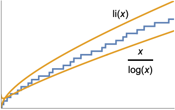
Plot[{PrimePi[x], x / Log[x], LogIntegral[x], RiemannR[x]}, {x, 1.5, 100}, Rule[...]]![]() is bounded below by
is bounded below by ![]() and is bounded above by
and is bounded above by ![]() for
for ![]() greater than 3:
greater than 3:
Plot[{x / Log[x], PrimePi[x], x / (Log[x] - 1.112)}, {x, 3, 100}, Rule[...]]Plot[{(x/HarmonicNumber[x] - 3 / 2), PrimePi[x]}, {x, 50, 200}, Rule[...]]![]() for
for ![]() if the Riemann hypothesis is true:
if the Riemann hypothesis is true:
Plot[{Abs[PrimePi[x] - LogIntegral[x]], Sqrt[x]Log[x] / (8 * Pi)}, {x, 2657, 3000}, PlotLegends -> "Expressions"]Count the prime numbers using EulerPhi:
primecount[x_] := Underoverscript[∑, k = 2, ⌊x⌋]⌊(EulerPhi[k]/k - 1)⌋Table[primecount[n], {n, 0, 10}]Table[PrimePi[n], {n, 0, 10}]Compute PrimePi based on the Hardy–Wright formula:
primecount[x_] := Sum[Mod[(j - 2)!, j], {j, 4, x}]Table[primecount[n], {n, 5, 10}]Table[PrimePi[n], {n, 5, 10}]Compute PrimePi using Accumulate:
Accumulate[Table[Boole[PrimeQ[n]], {n, 1, 10}]]Table[PrimePi[n], {n, 1, 10}]Number Theory (8)
Find twin primes up to ![]() , i.e. pairs of primes of the form
, i.e. pairs of primes of the form ![]() :
:
TwinPrimes[n_] := Pick[#, PrimeQ[# + 2]]&[Prime[Range[PrimePi[n]]]]TwinPrimes[100]TwinPrimePi[n_] := Length[Pick[#, PrimeQ[# + 2]]]&[Prime[Range[PrimePi[n]]]]Plot the sequence of twin primes and PrimePi:
ListStepPlot[{Table[TwinPrimePi[n], {n, 1, 100}], Table[PrimePi[n], {n, 1, 100}]}]The ![]()
![]() Ramanujan prime is the smallest number
Ramanujan prime is the smallest number ![]() such that
such that ![]() for all
for all ![]() :
:
list = Table[PrimePi[n] - PrimePi[n / 2], {n, 10 ^ 4}];ramanujanPrime = 1 + Last[Position[list, #]][[1]]& /@ Range[0, 50];ramanujanPrimePi[n_] := Count[ramanujanPrime, _ ? (# ≤ n&)]Plot the sequence of Ramanujan primes:
Plot[ramanujanPrimePi[n], {n, 0, 100}]Compare the count of Ramanujan primes to PrimePi:
Plot[{ramanujanPrimePi[n], PrimePi[n]}, {n, 0, 100}]Calculate the primorial up to the ![]()
![]() prime, i.e. a function that multiplies successive primes, similar to the factorial:
prime, i.e. a function that multiplies successive primes, similar to the factorial:
primorial[0] := 1
primorial[1] := 2
primorial[n_] := Times@@Prime@Range[n];primorial[5]Compare the primorial to the factorial up to ![]() :
:
DiscretePlot[{Log[n!], Log[Times@@Prime[Range[PrimePi[n]]]]}, {n, 1, 50}]Plot the differences between the factorial and the primorial up to ![]() :
:
ListLinePlot[If[True, Differences, Identity][Table[Log[(n!/Times@@Prime[Range[PrimePi[n]]])], {n, 1, 100, 1}]], Filling -> Axis]Plot the Chebyshev theta function:
chebyshevTheta[n_] := Log[primorial[PrimePi[n]]];Plot[chebyshevTheta[n], {n, 1, 100}]DiscretePlot[{chebyshevTheta[n], PrimePi[n]}, {n, 1, 100}]Calculate the prime powers up to ![]() :
:
primePowers[n_] := Union@@Table[Prime[Range[PrimePi[n ^ (1 / x)]]] ^ x, {x, Log2[n]}]primePowers[10]PrimePowerQ[%]Count all the prime powers up to ![]() :
:
primePowerPi[n_] := PrimePi[n] + Sum[Floor@Log[Prime[k], n] - 1, {k, PrimePi[Sqrt[n]//Floor]}]primePowerPi[10]Graph the count of prime powers:
DiscretePlot[primePowerPi[n], {n, 1, 100}]Compare the count of prime powers to PrimePi:
DiscretePlot[{primePowerPi[n], PrimePi[n]}, {n, 1, 100}]Visualize the second Hardy–Littlewood conjecture, which states that ![]() for
for ![]() :
:
ArrayPlot[((Outer[Plus, #, #]&)[PrimePi[Range[2, 20]]] - Outer[PrimePi[+##1]&, #, #]&)[Range[2, 20]], Rule[...]]Plot Brocard's conjecture, which states that if ![]() and
and ![]() are consecutive primes greater than 2, then between
are consecutive primes greater than 2, then between ![]() and
and ![]() there are at least four prime numbers:
there are at least four prime numbers:
ListStepPlot[-Subtract@@@Partition[PrimePi[Prime[Range[100]] ^ 2], 2, 1], Rule[...]]Find Goldbach partitions, i.e. pairs of primes (![]() ,
, ![]() ) such that
) such that ![]() :
:
goldbachPartitions[n_] := IntegerPartitions[2n, {2}, Prime[Range[PrimePi[2n]]]]goldbachPartitions[50]Graph Goldbach's conjecture/comet:
ListPlot[Transpose[{Range[4, 1000, 2], Length /@ Table[IntegerPartitions[i, 2, Table[Prime[n], {n, PrimePi[i]}]], {i, 4, 1000, 2}]}], Rule[...]]Cases[Range[100], n_ /; PrimePi[n] == EulerPhi[n]]DiscretePlot[{PrimePi[n], EulerPhi[n]}, {n, 1, 22}, Rule[...]]Properties & Relations (5)
The largest domain of definitions of PrimePi:
FunctionDomain[PrimePi[x], x, Complexes]PrimePi is asymptotically equivalent to ![]() as
as ![]() :
:
AsymptoticEquivalent[PrimePi[x], x / Log[x], x -> Infinity]And to LogIntegral:
AsymptoticEquivalent[PrimePi[x], LogIntegral[x], x -> Infinity]PrimePi is the inverse of Prime:
PrimePi[Prime[100]]Use PrimeQ to count prime numbers:
Count[Table[PrimeQ[n], {n, 1, 1000}], True]PrimePi[1000]Entity["MathematicalFunction", "PrimePi"]An integral representation of PrimePi:
Entity["MathematicalFunction", "PrimePi"]["IntegralRepresentations"]Possible Issues (1)
Neat Examples (3)
Ulam spiral colored based on the difference in PrimePi values:
ulam[n_] := Partition[Permute[Range[n ^ 2], Accumulate[Take[Flatten[{{n ^ 2 + 1} / 2, Table
[(-1) ^ j i, {j, n}, {i, {-1, n}}, {j}]}], n ^ 2]]], n]ArrayPlot[PrimePi[ulam[101] + 10] - PrimePi[ulam[101]], Rule[...]]Generate a path based on the PrimePi function:
Graphics[Line[AnglePath[Table[PrimePi[n], {n, 1, 1000}]], Rule[...]]]Construct polyhedra using directed graphs generated by primes less than ![]() :
:
vertexcoords[p_] :=
GraphEmbedding[Graph3D[Flatten[Table[i -> Mod[i * q, p], {i, 1, p - 1}, {q, Prime[Range[PrimePi[p] - 1]]}]]]]Table[ConvexHullMesh[vertexcoords[p], Rule[...]], {p, Prime[Range[4, 7]]}]Text
Wolfram Research (1991), PrimePi, Wolfram Language function, https://reference.wolfram.com/language/ref/PrimePi.html (updated 2021).
CMS
Wolfram Language. 1991. "PrimePi." Wolfram Language & System Documentation Center. Wolfram Research. Last Modified 2021. https://reference.wolfram.com/language/ref/PrimePi.html.
APA
Wolfram Language. (1991). PrimePi. Wolfram Language & System Documentation Center. Retrieved from https://reference.wolfram.com/language/ref/PrimePi.html