Wolfram Language & System Documentation Center

RadonTransform

gives the Radon transform of expr.

Details and Options

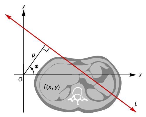
The Radon transform of a function is defined to be .
Geometrically, the Radon transform represents the integral of along a line given in normal form by the equation , with -∞<p<∞ and -π/2<ϕ<π/2.

The following options can be given:

Assumptions	$Assumptions	assumptions on parameters
GenerateConditions	False	whether to generate results that involve conditions on parameters
Method	Automatic	what method to use

In TraditionalForm, RadonTransform is output using .

Examples

open all close all

Basic Examples (1)

Compute the Radon transform of a function:

Wolfram Language code: RadonTransform[(x^2 + 5y^2) E^-x^2 - y^2, {x, y}, {p, ϕ}]

Plot the function along with the transform:

Wolfram Language code:

{DensityPlot[(x^2 + 5 y^2) E^-x^2 - y^2, {x, -2, 2}, {y, -2, 2}, Frame -> None, Ticks -> None], DensityPlot[%, {ϕ, -π / 2, π / 2}, {p, -3, 3}, Frame -> None, Ticks -> None]}

Scope (10)

Basic Uses (2)

Compute the Radon transform of a function for symbolic parameter values:

Wolfram Language code: RadonTransform[x E ^ (-x ^ 2 - y ^ 2), {x, y}, {p, ϕ}]

Use exact values for the parameters:

Wolfram Language code: RadonTransform[x E ^ (-x ^ 2 - y ^ 2), {x, y}, {3, π / 3}]

Use inexact values for the parameters:

Wolfram Language code: RadonTransform[x E ^ (-x ^ 2 - y ^ 2), {x, y}, {3.1, 0.8}]

Obtain the condition for validity of a Radon transform:

Wolfram Language code: RadonTransform[y E ^ (-a(x ^ 2 + y ^ 2)), {x, y}, {p, ϕ}, GenerateConditions -> True]

Specify assumptions:

Wolfram Language code: RadonTransform[y E ^ (-a(x ^ 2 + y ^ 2)), {x, y}, {p, ϕ}, GenerateConditions -> True, Assumptions -> a > 0]

Gaussian Functions (5)

Radon transform of a circular Gaussian function:

Wolfram Language code: RadonTransform[ E^-x^2 - y^2, {x, y}, {p, ϕ}]

Plot the function along with the transform:

Wolfram Language code:

{DensityPlot[E^-x^2 - y^2, {x, -2, 2}, {y, -2, 2}, Frame -> None, Ticks -> None], DensityPlot[%, {ϕ, -π / 2, π / 2}, {p, -2, 2}, Frame -> None, Ticks -> None]}

Radon transform of an elliptic Gaussian function:

Wolfram Language code: RadonTransform[E^-(x^2/25) - (y^2/16), {x, y}, {p, ϕ}]

Plot the function along with the transform:

Wolfram Language code:

{DensityPlot[E^-(x^2/25) - (y^2/16), {x, -3, 3}, {y, -3, 3}, Frame -> None, Ticks -> None, Frame -> None, Ticks -> None], DensityPlot[%, {ϕ, -π / 2, π / 2}, {p, -5, 5}, Frame -> None, Ticks -> None]}

Product of a polynomial with a Gaussian function:

Wolfram Language code: RadonTransform[(x^2 + y^2) E^-x^2 - y^2, {x, y}, {p, ϕ}]

Wolfram Language code:

{DensityPlot[(x^2 + y^2) E^-x^2 - y^2, {x, -2, 2}, {y, -2, 2}, Frame -> None, Ticks -> None], DensityPlot[%, {ϕ, -π / 2, π / 2}, {p, -5, 5}, Frame -> None, Ticks -> None]}

Product of Hermite polynomials and a Gaussian function:

Wolfram Language code: RadonTransform[HermiteH[1, x] HermiteH[2, y] E^-x^2 - y^2, {x, y}, {p, ϕ}]

Wolfram Language code:

{DensityPlot[HermiteH[1, x] HermiteH[2, y]  E^-x^2 - y^2, {x, -2, 2}, {y, -2, 2}, Frame -> None, Ticks -> None], DensityPlot[%, {ϕ, -π / 2, π / 2}, {p, -2, 2}, Frame -> None, Ticks -> None]}

Products of trigonometric functions with Gaussian functions:

Wolfram Language code: RadonTransform[Cos[x + y] E^-x^2 - y^2, {x, y}, {p, ϕ}]

Wolfram Language code:

{DensityPlot[Cos[x + y] E^-x^2 - y^2, {x, -2, 2}, {y, -2, 2}, PlotRange -> All, Frame -> None, Ticks -> None], DensityPlot[%, {ϕ, -π / 2, π / 2}, {p, -2, 2}, PlotRange -> All, Frame -> None, Ticks -> None]}

Wolfram Language code: RadonTransform[Sin[2x + y] E^-x^2 - y^2, {x, y}, {p, ϕ}]

Wolfram Language code:

{DensityPlot[Sin[2x + y]  E^-x^2 - y^2 , {x, -2, 2}, {y, -2, 2}, Frame -> None, Ticks -> None], DensityPlot[%, {ϕ, -π / 2, π / 2}, {p, -2, 2}, Frame -> None, Ticks -> None]}

Piecewise and Generalized Functions (3)

Radon transform of the characteristic function for the unit disk:

Wolfram Language code: RadonTransform[UnitStep[1 - x ^ 2 - y ^ 2], {x, y}, {p, ϕ}]

Wolfram Language code:

{DensityPlot[UnitStep[1 - x ^ 2 - y ^ 2], {x, -2, 2}, {y, -2, 2}, PlotRange -> All, PlotPoints -> 200, Frame -> None, Ticks -> None], DensityPlot[%, {ϕ, -π / 2, π / 2}, {p, -2, 2}, PlotRange -> All, PlotPoints -> 200, Frame -> None, Ticks -> None]}

Products of polynomials with the characteristic function for the unit disk:

Wolfram Language code: RadonTransform[x UnitStep[1 - x ^ 2 - y ^ 2], {x, y}, {p, ϕ}]

Wolfram Language code:

{DensityPlot[x UnitStep[1 - x ^ 2 - y ^ 2], {x, -2, 2}, {y, -2, 2}, PlotRange -> All, PlotPoints -> 200, Frame -> None, Ticks -> None], DensityPlot[%, {ϕ, -π / 2, π / 2}, {p, -2, 2}, PlotRange -> All, PlotPoints -> 200, Frame -> None, Ticks -> None]}

Wolfram Language code: RadonTransform[(x ^ 2 + y ^ 2) UnitStep[1 - x ^ 2 - y ^ 2], {x, y}, {p, ϕ}]

Wolfram Language code:

{DensityPlot[(x ^ 2 + y ^ 2) UnitStep[1 - x ^ 2 - y ^ 2], {x, -2, 2}, {y, -2, 2}, PlotRange -> All, PlotPoints -> 200, Frame -> None, Ticks -> None], DensityPlot[%, {ϕ, -π / 2, π / 2}, {p, -2, 2}, PlotRange -> All, PlotPoints -> 200, Frame -> None, Ticks -> None]}

Radon transforms for expressions involving DiracDelta:

Wolfram Language code: RadonTransform[DiracDelta[x - a, y - b], {x, y}, {p, ϕ}]

Wolfram Language code: RadonTransform[x DiracDelta[1 - x ^ 2 - y ^ 2], {x, y}, {p, ϕ}]

Options (2)

Assumptions (1)

Specify assumptions:

Wolfram Language code: RadonTransform[UnitStep[1 - x ^ 2 - y ^ 2], {x, y}, {p, ϕ}]

Wolfram Language code: RadonTransform[UnitStep[1 - x ^ 2 - y ^ 2], {x, y}, {p, ϕ}, Assumptions -> -1 < p < 1]

GenerateConditions (1)

Generate conditions for the validity of the result:

Wolfram Language code: RadonTransform[x E ^ (-a(x ^ 2 + y ^ 2)), {x, y}, {p, ϕ}]

Wolfram Language code: RadonTransform[x E ^ (-a(x ^ 2 + y ^ 2)), {x, y}, {p, ϕ}, GenerateConditions -> True]

Applications (2)

Compute the symbolic Radon transform for the characteristic function of a disk:

Wolfram Language code: RadonTransform[UnitStep[1 - x ^ 2 - y ^ 2], {x, y}, {p, ϕ}]

Wolfram Language code:

{DensityPlot[UnitStep[1 - x ^ 2 - y ^ 2], {x, -2, 2}, {y, -2, 2}, PlotRange -> All, PlotPoints -> 200, Frame -> None, Ticks -> None, Background -> None], DensityPlot[%, {ϕ, -π / 2, π / 2}, {p, -Sqrt[8], Sqrt[8]}, PlotRange -> All, Frame -> None, Ticks -> None, Background -> None]}

Obtain the same result using Radon:

Wolfram Language code: disk = Image[DiskMatrix[50, 201], "Bit"];

Wolfram Language code: {disk, Radon[disk, {201, 201}]}

Use the Radon transform to solve a Poisson equation:

Wolfram Language code: peqn = Laplacian[u[x, y], {x, y}] == E^-x^2 - y^2 x (-2 + x^2 + y^2);

Apply RadonTransform to the equation:

Wolfram Language code: RadonTransform[peqn, {x, y}, {p, m}]

Solve the ordinary differential equation using DSolveValue:

Wolfram Language code: DSolveValue[% /. {RadonTransform[u[x, y], {x, y}, {p, m}] -> f[p]}, f[p], p]

Set the arbitrary constants in the solution to 0:

Wolfram Language code: % /. {C[i_] -> 0}

Obtain the solution for the original equation using InverseRadonTransform:

Wolfram Language code: sol = InverseRadonTransform[%, {p, m}, {x, y}]

Verify the solution:

Wolfram Language code: peqn /. {u -> Function[{x, y}, Evaluate[sol]]}//Simplify

Plot the solution:

Wolfram Language code: Plot3D[sol, {x, -3, 3}, {y, -3, 3}, PlotRange -> All]

Properties & Relations (10)

RadonTransform computes the integral :

Wolfram Language code: RadonTransform[E^-x^2 - y^2, {x, y}, {p, ϕ}]

Obtain the same result using Integrate:

Wolfram Language code: f[x_, y_] := E^-x^2 - y^2

Wolfram Language code: Subsuperscript[∫, -∞, ∞]f[p Cos[ϕ] - s Sin[ϕ], p Sin[ϕ] + s Cos[ϕ]]ⅆs

RadonTransform and InverseRadonTransform are mutual inverses:

Wolfram Language code: InverseRadonTransform[RadonTransform[f[x, y], {x, y}, {p, ϕ}], {p, ϕ}, {x, y}]

Wolfram Language code: RadonTransform[InverseRadonTransform[g[p, ϕ], {p, ϕ}, {x, y}], {x, y}, {p, ϕ}]

RadonTransform is a linear operator:

Wolfram Language code: RadonTransform[a f[x, y] + b g[x, y], {x, y}, {p, ϕ}]

The shifting property for RadonTransform:

Wolfram Language code: f[x_, y_] := E ^ (-x ^ 2 - y ^ 2)

Wolfram Language code: a = 2;b = 5;

Wolfram Language code: RadonTransform[f[x - a, y - b], {x, y}, {p, ϕ}] == RadonTransform[f[x, y], {x, y}, {p - a Cos[ϕ] - b Sin[ϕ], ϕ}]

The symmetry property for RadonTransform:

Wolfram Language code: f[x_, y_] := E ^ (-x ^ 2 / 25 - y ^ 2 / 16)

Wolfram Language code: a = 2;b = 5;

Express the Radon transform of in terms of a unit vector:

Wolfram Language code:

s1 = RadonTransform[f[x, y], {x, y}, {p, ϕ}] /. {Sin[a_] :> TrigExpand[Sin[a]]} /. {Cos[ϕ] -> Subscript[u, 1], Sin[ϕ] -> Subscript[u, 2]}

Verify the symmetry property:

Wolfram Language code: (s1 /. {p -> -p, Subscript[u, 1] -> -Subscript[u, 1], Subscript[u, 2] -> -Subscript[u, 2]}) == s1//Simplify

The homogeneity property for RadonTransform:

Wolfram Language code: f[x_, y_] := E ^ (-x ^ 2 / 25 - y ^ 2 / 16)

Wolfram Language code: a = 2;b = 5;

Express the Radon transform of in terms of a unit vector:

Wolfram Language code:

s1 = RadonTransform[f[x, y], {x, y}, {p, ϕ}] /. {Sin[a_] :> TrigExpand[Sin[a]]} /. {Cos[ϕ] -> Subscript[u, 1], Sin[ϕ] -> Subscript[u, 2]}

Verify the homogeneity property:

Wolfram Language code: k = 7;

Wolfram Language code:

(s1  /. {p -> k p, Subscript[u, 1] -> k Subscript[u, 1], Subscript[u, 2] -> k Subscript[u, 2]}) == 1 / Abs[k] s1//Simplify

The scaling property for RadonTransform:

Wolfram Language code: f[x_, y_] := E ^ (-x ^ 2 / 25 - y ^ 2 / 16)

Wolfram Language code: a = 2;b = 5;

Express the Radon transform of in terms of a unit vector:

Wolfram Language code:

s1 = RadonTransform[f[x, y], {x, y}, {p, ϕ}] /. {Sin[a_] :> TrigExpand[Sin[a]]} /. {Cos[ϕ] -> Subscript[u, 1], Sin[ϕ] -> Subscript[u, 2]}

Express the Radon transform of in terms of a unit vector:

Wolfram Language code:

s2 = RadonTransform[f[a x, b y], {x, y}, {p, ϕ}] /. {Sin[a_] :> TrigExpand[Sin[a]]} /. {Cos[ϕ] -> Subscript[u, 1], Sin[ϕ] -> Subscript[u, 2]}

Verify the scaling property:

Wolfram Language code: 1 / Abs[a b] (s1 /. {Subscript[u, 1] -> Subscript[u, 1] / a, Subscript[u, 2] -> Subscript[u, 2] / b}) == s2//Simplify

RadonTransform of derivatives:

Wolfram Language code: RadonTransform[D[f[x, y], x], {x, y}, {p, ϕ}]

Wolfram Language code: RadonTransform[D[f[x, y], y], {x, y}, {p, ϕ}]

RadonTransform of the Laplacian:

Wolfram Language code: RadonTransform[Laplacian[f[x, y], {x, y}], {x, y}, {p, ϕ}]

RadonTransform can be computed using Fourier transforms:

Wolfram Language code: f[x_, y_] := (x ^ 2 + y ^ 2)E ^ (-Pi(x ^ 2 + y ^ 2))

Compute the Fourier transform of f in polar coordinates:

Wolfram Language code: FourierTransform[f[x, y], {x, y}, {u, v}, FourierParameters -> {0, -2Pi}] /. {u -> r Cos[ϕ], v -> r Sin[ϕ]}//Simplify

Compute the inverse Fourier transform to obtain the Radon transform:

Wolfram Language code: InverseFourierTransform[%, r, p, FourierParameters -> {0, -2Pi}]

Obtain the same result directly using RadonTransform:

Wolfram Language code: RadonTransform[f[x, y], {x, y}, {p, ϕ}]

Neat Examples (1)

Create a table of basic Radon transforms:

Wolfram Language code:

flist = {E ^ (-x ^ 2 - y ^ 2), x  E ^ (-x ^ 2 - y ^ 2), y  E ^ (-x ^ 2 - y ^ 2), (x ^ 2 + y ^ 2) E ^ (-x ^ 2 - y ^ 2), E ^ (-(x / a) ^ 2 - (y / b) ^ 2), DiracDelta[x - a, y - b], UnitStep[1 - x ^ 2 - y ^ 2], (x ^ 2 + y ^ 2)UnitStep[1 - x ^ 2 - y ^ 2]};

Wolfram Language code:

Grid[Prepend[{#, RadonTransform[#1, {x, y}, {p, ϕ}]}& /@ flist, {"Function", "Radon Transform"}], IconizedObject[«Grid options»]]//TraditionalForm

Top

More Learning

Tech Support

Wolfram Solutions

Wolfram Solutions For Education

Get Started

Grow Your Skills

Work with Us

Educational Programs for Adults

Educational Programs for Youth

Read

RadonTransform

Details and Options

Examples

Basic Examples (1)

Scope (10)

Basic Uses (2)

Gaussian Functions (5)

Piecewise and Generalized Functions (3)

Options (2)

Assumptions (1)

GenerateConditions (1)

Applications (2)

Properties & Relations (10)

Neat Examples (1)

Text

CMS

APA

BibTeX

BibLaTeX

RadonTransform

Details and Options

Examples

Basic Examples (1)

Scope (10)

Basic Uses (2)

Gaussian Functions (5)

Piecewise and Generalized Functions (3)

Options (2)

Assumptions (1)

GenerateConditions (1)

Applications (2)

Properties & Relations (10)

Neat Examples (1)

See Also

Related Guides

History

Text

CMS

APA

BibTeX

BibLaTeX