

WattsStrogatzGraphDistribution
WattsStrogatzGraphDistribution[n,p]
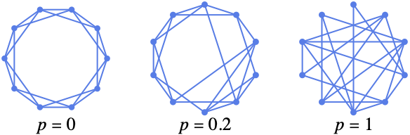
represents the Watts–Strogatz graph distribution for n-vertex graphs with rewiring probability p.
WattsStrogatzGraphDistribution[n,p,k]
represents the Watts–Strogatz graph distribution for n-vertex graphs with rewiring probability p starting from a 2k-regular graph.
Details
- WattsStrogatzGraphDistribution is also known as small-world graph distribution.
- WattsStrogatzGraphDistribution[n,p] is equivalent to WattsStrogatzGraphDistribution[n,p,2].
- The WattsStrogatzGraphDistribution is constructed starting from CirculantGraph[n,Range[k]] and rewiring each edge with probability p. Each edge is rewired by changing one of the vertices, making sure that no loop or multiple edge is created.
- WattsStrogatzGraphDistribution can be used with such functions as RandomGraph and GraphPropertyDistribution.
Examples
open all close allBasic Examples (2)
Generate a pseudorandom graph:
RandomGraph[WattsStrogatzGraphDistribution[50, 0.05]]GlobalClusteringCoefficient as a function of rewiring probability:
ListLogLinearPlot[Table[{p, GlobalClusteringCoefficient[RandomGraph[WattsStrogatzGraphDistribution[10 ^ 3, p, 5]]]}, {p, 10 ^ Range[-4, 0, 0.05]}], Joined -> True]Scope (3)
Generate simple undirected graphs:
RandomGraph[WattsStrogatzGraphDistribution[30, 0.03, 3]]Generate a set of pseudorandom graphs:
RandomGraph[WattsStrogatzGraphDistribution[20, 0.07], 4]Compute probabilities and statistical properties:
𝒟 = GraphPropertyDistribution[GlobalClusteringCoefficient[g], gWattsStrogatzGraphDistribution[10, 0.2]];NExpectation[x, x𝒟]Applications (3)
The Western States Power Grid can be modeled with WattsStrogatzGraphDistribution:
g = ExampleData[{"NetworkGraph", "PowerGrid"}];𝒢 = WattsStrogatzGraphDistribution[VertexCount[g], 0.25, Round[EdgeCount[g] / VertexCount[g]]]The model captures the small-world characteristics of the empirical network, with short mean graph distance and high clustering:
{N[MeanGraphDistance[g]], N[MeanClusteringCoefficient[g]]}h = RandomGraph[WattsStrogatzGraphDistribution[10 ^ 3, 0.25, 2]];{N[MeanGraphDistance[h]], N[MeanClusteringCoefficient[h]]}A social network in a village of 100 people where the average number of relations per person is 20 can be modeled using a WattsStrogatzGraphDistribution. Find the expected number of relations for the least-connected person:
𝒢 = WattsStrogatzGraphDistribution[100, 0.1, 20 / 2];g = RandomGraph[𝒢]The expected number of relations for the least-connected person:
𝒟 = GraphPropertyDistribution[Min[VertexDegree[h]], h𝒢];
NExpectation[x, x𝒟]𝒟 = GraphPropertyDistribution[GraphDiameter[h], h𝒢];Round[N[Mean[𝒟]]]This represents a simplified model for the spread of an infectious disease in a social network. The disease spreads in each step with probability 0.4 from infected individuals to some of their susceptible neighbors, while infected individuals recover and become immune:
network = RandomGraph[WattsStrogatzGraphDistribution[100, 0.1, 3]]Simulate an infection and find infected persons:
infect[z_, p_] := Pick[z, RandomChoice[{p, 1 - p} -> {1, 0}, Length[z]], 1];
step[g_, {i_, q_}, p_] :=
	{Complement[infect[AdjacencyList[g, i], p], i, q], Join[q, i]};
infected[g_, i_, p_] := Last[FixedPoint[step[g, #, p]&, {i, {}}]]infected[network, {1}, 0.4] //ShortHighlightGraph[network, %]The fraction of infected persons as a function of the transmission probability:
count[p_] := Mean[Table[Length[infected[network, {1}, p]], {100}]];DiscretePlot[count[p], {p, 0, 1, 0.1}, Joined -> True]Properties & Relations (5)
Distribution of the number of vertices:
GraphPropertyDistribution[VertexCount[g], gWattsStrogatzGraphDistribution[n, p, k]]Distribution of the number of edges:
GraphPropertyDistribution[EdgeCount[g], gWattsStrogatzGraphDistribution[n, p, k]]Distribution of the vertex degree:
𝒟[n_, p_, k_] := HistogramDistribution[Flatten[Table[VertexDegree[g], {g, RandomGraph[WattsStrogatzGraphDistribution[n, p, k], 1000]}]], {-1 / 2, n, 1}];DiscretePlot[Evaluate@Table[PDF[𝒟[50, p, 2], d], {p, 0, 1, 1 / 3}], {d, 0, 8}, PlotRange -> All, ExtentSize -> 4 / 5]Approximate with a sum of BinomialDistribution and PoissonDistribution:
ℱ[n_, p_, k_] := TransformedDistribution[x + y, {xBinomialDistribution[2k, 1 - p / 2], yPoissonDistribution[k p]}]DiscretePlot[Evaluate@{PDF[𝒟[100, 0.4, 3], d], PDF[ℱ[100, 0.4, 3], d]}, {d, 0, 15}, PlotRange -> All, ExtentSize -> 4 / 5]The mean distance decreases quickly as the rewiring probability increases:
ListLogLinearPlot[Table[{p, MeanGraphDistance[RandomGraph[WattsStrogatzGraphDistribution[10 ^ 3, p, 5]]]}, {p, Table[10 ^ x, {x, -3, 0, 0.3}]}], Joined -> True, PlotRange -> All]The clustering coefficient decreases slowly:
ListLogLinearPlot[Table[{p, GlobalClusteringCoefficient[RandomGraph[WattsStrogatzGraphDistribution[10 ^ 3, p, 5]]]}, {p, Table[10 ^ x, {x, -3, 0, 0.3}]}], Joined -> True]WattsStrogatzGraphDistribution[n,0,k] is a 2k-regular graph:
RandomGraph[WattsStrogatzGraphDistribution[13, 0, 6]]VertexDegree[%]RandomGraph[WattsStrogatzGraphDistribution[12, 0, 6]]VertexDegree[%]Text
Wolfram Research (2010), WattsStrogatzGraphDistribution, Wolfram Language function, https://reference.wolfram.com/language/ref/WattsStrogatzGraphDistribution.html.
CMS
Wolfram Language. 2010. "WattsStrogatzGraphDistribution." Wolfram Language & System Documentation Center. Wolfram Research. https://reference.wolfram.com/language/ref/WattsStrogatzGraphDistribution.html.
APA
Wolfram Language. (2010). WattsStrogatzGraphDistribution. Wolfram Language & System Documentation Center. Retrieved from https://reference.wolfram.com/language/ref/WattsStrogatzGraphDistribution.html