"NeighborhoodContraction" (Machine Learning Method)
- Method for FindClusters, ClusterClassify and ClusteringComponents.
- Partitions data into clusters of similar elements using the "NeighborhoodContraction" clustering algorithm.
Details & Suboptions
- "NeighborhoodContraction" is a neighbor-based clustering method. "NeighborhoodContraction" works for arbitrary cluster shapes and sizes, however, it can fail when clusters have different densities or are intertwined.
- The following plots show the results of the "NeighborhoodContraction" method applied to toy datasets:
-
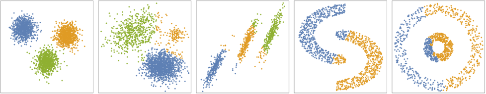
- The "NeighborhoodContraction" method iteratively shifts data points toward higher density regions. During this procedure, data points tend to collapse to different fixed points, each of them representing a cluster.
- Formally, at each step, each data point
 is set to the mean of its neighboring points
  ,
, 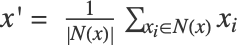 .
. - Neighboring points
 are defined as all the points within a ball of ϵ radius. The algorithm repeats the updates until points stop moving; all points belonging to a cluster are then collapsed (up to a tolerance). This algorithm is equivalent to the "MeanShift" method but with a different neighborhood definition.
 - The following suboption can be given:
-
"NeighborhoodRadius" Automatic radius ϵ
Examples
open all close allBasic Examples (3)
Find clusters of nearby values using the "NeighborhoodContraction" clustering method:
FindClusters[{1, 2, 10, 12, 3, 1, 13, 25, 27, 28}, Method -> "NeighborhoodContraction"]Train the ClassifierFunction on a list of colors using the "NeighborhoodContraction" method:
SeedRandom[12];
colors = RandomColor[200];
c = ClusterClassify[colors, Method -> "NeighborhoodContraction"]
Gather the elements by their class number:
GatherBy[colors, c]Train a ClassifierFunction on a mixture of two-dimensional normal distributions:
ns = 600;
Gaussiandata[ns_, mean_, cov_] :=
	BlockRandom[RandomVariate[MultinormalDistribution[mean, cov], ns]];

data = Join[Gaussiandata[1200, {0, 0},   {{1, 0 }, {0 , 1}}], Gaussiandata[600, {1.5, 4.5},   {{1, 0 }, {0 , 1}}] ,
	Gaussiandata[300, {-3, 5}, {{2, 1 / 2 }, {1 / 2 , 2}}]];

cl = ClusterClassify[data, Method -> "NeighborhoodContraction"]
Find the cluster assignments and visualize them:
decision = cl[data];
classes = Information[cl, "Classes"];ListPlot[Pick[data, decision, #]& /@ classes]
Options (3)
DistanceFunction (2)
Generate a list of 200 random colors:
SeedRandom[12];
colors = RandomColor[200]
Find clusters by specifying a DistanceFunction option:
FindClusters[colors, Method -> "NeighborhoodContraction", DistanceFunction -> ColorDistance]Generate points based on a mixture of two-dimensional normal distributions:
ns = 600;
Gaussiandata[ns_, mean_, cov_] :=
	BlockRandom[RandomVariate[MultinormalDistribution[mean, cov], ns]];

data = Join[Gaussiandata[1200, {0, 0},   {{1, 0 }, {0 , 1}}], Gaussiandata[600, {1.5, 4.5},   {{1, 0 }, {0 , 1}}] ,
	Gaussiandata[300, {-2, 5}, {{2, 1 / 2 }, {1 / 2 , 2}}]];
Find different clustering structures by specifying different DistanceFunction options:
Grid[{Table[ListPlot[FindClusters[data, Method -> {"NeighborhoodContraction"}, DistanceFunction -> df],
	Frame -> True, Axes -> False, FrameTicks -> None, AspectRatio -> 1, PlotStyle -> Directive[PointSize[0.03]]], {df, {EuclideanDistance, ChessboardDistance, ManhattanDistance}}]
	}]
"NeighborhoodRadius" (1)
Generate points based on a mixture of two-dimensional normal distributions:
ns = 600;
Gaussiandata[ns_, mean_, cov_] :=
	BlockRandom[RandomVariate[MultinormalDistribution[mean, cov], ns]];

data = Join[Gaussiandata[1200, {0, 0},   {{1, 0 }, {0 , 1}}], Gaussiandata[600, {1.5, 4.5},   {{1, 0 }, {0 , 1}}] ,
	Gaussiandata[300, {-2, 5}, {{2, 1 / 2 }, {1 / 2 , 2}}]];
Find different clustering structures by specifying different "NeighborhoodRadius" suboptions:
Grid[{Table[ListPlot[FindClusters[data, Method -> {"NeighborhoodContraction", "NeighborhoodRadius" -> nr}],
	Frame -> True, Axes -> False, FrameTicks -> None, AspectRatio -> 1, PlotStyle -> Directive[PointSize[0.03]]], {nr, {.1, .2, .4}}]
	}]