

BiquadraticFilterModel
BiquadraticFilterModel[{ω,q}]
creates a lowpass biquadratic filter using the characteristic frequency ω and the quality factor q.
BiquadraticFilterModel[{"type",spec}]
creates a filter of a given {"type",spec}.
BiquadraticFilterModel[{"type",spec},var]
expresses the model in terms of the variable var.
Details
- Biquadratic filters are second-order filters defined by a ratio of two quadratic polynomials. They are among the most commonly used circuits in analog and digital signal processing.
- BiquadraticFilterModel returns the filter as a TransferFunctionModel.
- Filter specifications {"type",spec} can be any of the following:
-
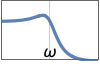
{"Lowpass",{{ω,q}}} uses cutoff frequency ω and quality factor q 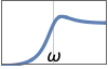
{"Highpass",{{ω,q}}} uses cutoff frequency ω and quality factor q 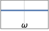
{"Allpass",{{ω,q}}} uses frequency ω and quality factor q 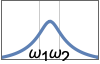
{"Bandpass",{ω1,ω2}} uses corner frequencies ω1 and ω2 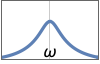
{"Bandpass",{{ω,q}}} uses center frequency ω and quality factor q 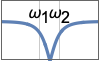
{"Bandstop",{ω1,ω2}} uses corner frequencies ω1 and ω2 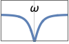
{"Bandstop",{{ω,q}}} uses center frequency ω and quality factor q - The following filter specifications can be given to create equalizers:
-
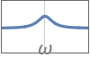
{"Peaking",{{ω,q}},g} peaking equalizer using gain value g 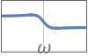
{"LowShelf",{{ω,q}},g} lowpass shelving equalizer using gain value g 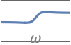
{"HighShelf",{{ω,q}},g} highpass shelving equalizer using gain value g - Given the gain value
 , the attenuation is
  .
.
Examples
open all close allBasic Examples (3)
tf = BiquadraticFilterModel[{1, 1}]BodePlot[tf, GridLines -> Automatic, PlotLayout -> "Magnitude"]A bandpass filter using the full specification:
tf = BiquadraticFilterModel[{"Bandpass", {{1, 1}}}]BodePlot[tf, {0.1, 10}, GridLines -> Automatic, PlotLayout -> "Magnitude"]Create a lowpass filter and apply it to a dual-tone signal:
in = Sin[ 1 / 5 t] + Sin[5t];
out = OutputResponse[BiquadraticFilterModel[{1, 1}], in, {t, 0, 60}];
Plot[{in, out}, {t, 0, 40}, PlotLegends -> {"Input", "Output"}]
Scope (8)
A symbolic lowpass filter with cutoff frequency ω and quality factor ![]() :
:
BiquadraticFilterModel[{ω, Q}]BiquadraticFilterModel[{"Lowpass", {{1, 1}}}, s]tf = BiquadraticFilterModel[{"Lowpass", {{10, 1}}}, s]BodePlot[tf, {1, 100}, GridLines -> Automatic, PlotLayout -> "Magnitude"]A symbolic highpass filter with cutoff frequency ![]() and quality factor
and quality factor ![]() :
:
BiquadraticFilterModel[{"Highpass", {{ω, Q}}}]tf = BiquadraticFilterModel[{"Highpass", {{10, 1}}}, s]BodePlot[tf, {1, 100}, GridLines -> Automatic, PlotLayout -> "Magnitude"]A symbolic bandpass filter with center frequency ![]() and quality factor
and quality factor ![]() :
:
BiquadraticFilterModel[{"Bandpass", {{ω, Q}}}]tf = BiquadraticFilterModel[{"Bandpass", {{1, 10}}}, s]BodePlot[tf, {0.1, 10}, GridLines -> Automatic, PlotLayout -> "Magnitude"]A symbolic bandstop filter with center frequency ![]() and quality factor
and quality factor ![]() :
:
BiquadraticFilterModel[{"Bandstop", {{ω, Q}}}]tf = BiquadraticFilterModel[{"Bandstop", {{1, 2}}}, s]BodePlot[tf, {0.1, 10}, PlotRange -> {0, -10}, GridLines -> Automatic, PlotLayout -> "Magnitude"]A symbolic allpass filter with center frequency ![]() and quality factor
and quality factor ![]() :
:
BiquadraticFilterModel[{"Allpass", {{ω, Q}}}]tf = BiquadraticFilterModel[{"Allpass", {{1, 2}}}, s]BodePlot[tf, PlotRange -> {0.99, 1.01}, PlotLayout -> "Magnitude"]A symbolic "Peaking" allpass filter with center frequency ![]() , quality factor
, quality factor ![]() , and gain value
, and gain value ![]() :
:
BiquadraticFilterModel[{"Peaking", {{ω, Q}}, g}]Use peak gain value of ![]() decibels:
decibels:
tf = BiquadraticFilterModel[{"Peaking", {{1, 1}}, Quantity[10, "dB"]}, s]BodePlot[tf, {0.1, 10}, PlotRange -> {-5, 15}, GridLines -> Automatic, PlotLayout -> "Magnitude"]A symbolic "LowShelf" filter with center frequency ![]() , quality factor
, quality factor ![]() , and gain value
, and gain value ![]() :
:
BiquadraticFilterModel[{"LowShelf", {{ω, Q}}, g}]Use low-shelf gain value of ![]() decibels:
decibels:
tf = BiquadraticFilterModel[{"LowShelf", {{1, 1}}, Quantity[-5, "dB"]}, s]BodePlot[tf, {0.1, 10}, PlotRange -> {-10, 10}, GridLines -> Automatic, PlotLayout -> "Magnitude"]A symbolic "HighShelf" filter with center frequency ![]() , quality factor
, quality factor ![]() , and gain value
, and gain value ![]() :
:
BiquadraticFilterModel[{"HighShelf", {{ω, Q}}, g}]Use low-shelf gain value of ![]() decibels:
decibels:
tf = BiquadraticFilterModel[{"HighShelf", {{1, 1}}, Quantity[-5, "dB"]}, s]BodePlot[tf, {0.1, 10}, PlotRange -> {-10, 10}, GridLines -> Automatic, PlotLayout -> "Magnitude"]Generalizations & Extensions (1)
Improve stopband attenuation by connecting two or more filters in series:
tf = BiquadraticFilterModel[{"Lowpass", {{1, 1}}}];
tfs = NestList[SystemsModelSeriesConnect[tf, #]&, tf, 2]BodePlot[tfs, {0.1, 10}, PlotRange -> {-120, 20}, GridLines -> Automatic, PlotLayout -> "Magnitude", FrameTicks -> {{Range[0, -120, -40], None}, {Automatic, Automatic}}, PlotLegends -> {"40 dB/decade", "80 dB/decade", "120 dB/decade"}]Applications (1)
Filter out the high-frequency tone in a pair of sinusoidal tones:
in = (Sin[ 1 / 5 t] + Sin[5t]) UnitStep[t];
Plot[in, {t, 20, 60}]
Use a biquadratic lowpass filter:
tf = BiquadraticFilterModel[{"Lowpass", {{1, 1}}}];
out = OutputResponse[tf, in, {t, 0, 60}];
Plot[out, {t, 20, 60}]
Create a higher-order filter by combining three filters to improve the filtering quality:
tf2 = Nest[SystemsModelSeriesConnect[tf, #]&, tf, 2]out = OutputResponse[tf2, in, {t, 0, 60}];
Plot[out, {t, 20, 60}]Properties & Relations (7)
Phase responses of the four basic filter types:
type = {"Lowpass", "Highpass", "Bandpass", "Bandstop"};
tfs = BiquadraticFilterModel[{#, {{1, 1}}}]& /@ type;
BodePlot[tfs, {0.1, 10.}, PlotLayout -> "Phase", GridLines -> Automatic, PlotLegends -> type]
Extract the order of a BiquadraticFilterModel:
SystemsModelOrder[StateSpaceModel[BiquadraticFilterModel[{"Lowpass", {{1., 1.}}}]]]Stop-band attenuation increases by a factor of 40 decibels per decade:
tf = BiquadraticFilterModel[{"Lowpass", {{1, 1}}}];
BodePlot[tf, {0.1, 10}, GridLines -> Automatic, PlotLayout -> "Magnitude"]
Gain at cutoff frequency increases with increasing values of quality factor ![]() :
:
tf = BiquadraticFilterModel[{"Lowpass", {{1, #}}}]& /@ {1 / 2, 1, 3, 9};
BodePlot[tf, {0.1, 10}, GridLines -> Automatic, PlotRange -> {-20, 20}, PlotLayout -> "Magnitude", PlotLegends -> {0.5, 1., 3., 9.}]
Width of bandpass filter decreases with increasing quality factor ![]() :
:
tf = BiquadraticFilterModel[{"Bandpass", {{1., #}}}]& /@ {0.5, 1., 3.};
BodePlot[tf, {0.1, 10}, GridLines -> Automatic, PlotLayout -> "Magnitude", PlotRange -> {-40, 5}, PlotLegends -> {0.5, 1., 3.}]
Gain values ![]() "boost" magnitude response of peaking equalizer:
"boost" magnitude response of peaking equalizer:
tfboost = BiquadraticFilterModel[{"Peaking", {{1, 1}}, #}, s]& /@ {4 / 3, 5 / 3, 6 / 3}BodePlot[tfboost, {0.1, 10}, PlotRange -> {-15, 15}, PlotLayout -> "Magnitude", GridLines -> Automatic, PlotLegends -> N@{4 / 3, 5 / 3, 6 / 3}]Gain values ![]() "cut" magnitude response of peaking equalizer:
"cut" magnitude response of peaking equalizer:
tfcut = BiquadraticFilterModel[{"Peaking", {{1, 1}}, #}, s]& /@ {3 / 6, 3 / 5, 3 / 4}BodePlot[tfcut, {0.1, 10}, PlotRange -> {-15, 15}, PlotLayout -> "Magnitude", GridLines -> Automatic, PlotLegends -> N@{3 / 6, 3 / 5, 3 / 4}]Gain values ![]() "boost" magnitude response of the low-shelf filter:
"boost" magnitude response of the low-shelf filter:
tfboost = BiquadraticFilterModel[{"LowShelf", {{1, 1}}, #}, s]& /@ {4 / 3, 5 / 3, 6 / 3}BodePlot[tfboost, {0.1, 10}, PlotRange -> {-15, 15}, PlotLayout -> "Magnitude", GridLines -> Automatic, PlotLegends -> N@{4 / 3, 5 / 3, 6 / 3}]Gain values ![]() "cut" magnitude response of the low-shelf filter:
"cut" magnitude response of the low-shelf filter:
tfcut = BiquadraticFilterModel[{"LowShelf", {{1, 1}}, #}, s]& /@ {3 / 6, 3 / 5, 3 / 4}BodePlot[tfcut, {0.1, 10}, PlotRange -> {-15, 15}, PlotLayout -> "Magnitude", GridLines -> Automatic, PlotLegends -> N@{3 / 6, 3 / 5, 3 / 4}]Text
Wolfram Research (2016), BiquadraticFilterModel, Wolfram Language function, https://reference.wolfram.com/language/ref/BiquadraticFilterModel.html.
CMS
Wolfram Language. 2016. "BiquadraticFilterModel." Wolfram Language & System Documentation Center. Wolfram Research. https://reference.wolfram.com/language/ref/BiquadraticFilterModel.html.
APA
Wolfram Language. (2016). BiquadraticFilterModel. Wolfram Language & System Documentation Center. Retrieved from https://reference.wolfram.com/language/ref/BiquadraticFilterModel.html