

Chebyshev1FilterModel
creates a lowpass Chebyshev type 1 filter of order n.
Chebyshev1FilterModel[{n,ωc}]
uses the cutoff frequency ωc.
Chebyshev1FilterModel[{"type",spec}]
creates a filter of a given "type" using the specified parameters spec.
Chebyshev1FilterModel[{"type",spec},var]
expresses the model in terms of the variable var.
Details
- Chebyshev1FilterModel returns the filter as a TransferFunctionModel.
- Chebyshev1FilterModel[{n,ω}] returns a lowpass filter with attenuation of
 (approximately 3 dB) at frequency ω.
 - Chebyshev1FilterModel[n] uses the cutoff frequency of 1.
- Lowpass filter specification {"type",spec} can be any of the following:
-
{"Lowpass",n} lowpass filter of order n and cutoff frequency 1 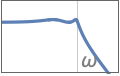
{"Lowpass",n,ωp} use cutoff frequency ωp 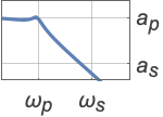
{"Lowpass",{ωp,ωs},{ap,as}} use full filter specification giving passband and stopband frequencies and attenuations - Highpass filter specifications:
-
{"Highpass",n} highpass filter with cutoff frequency 1 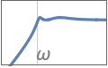
{"Highpass",n,ωp} use cutoff frequency ωp 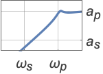
{"Highpass",{ωs,ωp},{as,ap}} full filter specification - Bandpass filter specifications:
-
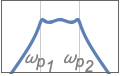
{"Bandpass",n,{ωp1,ωp2}} bandpass filter with passband frequencies ωp1 and ωp2 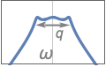
{"Bandpass",n,{{ω,q}}} use center frequency ω and quality factor q 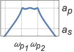
{"Bandpass",{ωs1,ωp1,ωp2,ωs2},{as,ap}} full filter specification - Bandstop filter specifications:
-
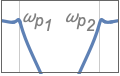
{"Bandstop",n,{ωp1,ωp2}} bandstop filter with passband frequencies ωp1 and ωp2 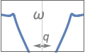
{"Bandstop",n,{{ω,q}}} use center frequency ω and quality factor q 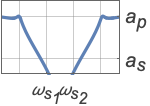
{"Bandstop",{ωp1,ωs1,ωs2,ωp2},{ap,as}} full filter specification - Frequency values should be given in an ascending order.
- Values ap and as are respectively absolute values of passband and stopband attenuations.
- Given a gain fraction
 , the attenuation is
  .
. - The quality factor q is defined as
 , with ω being the center frequency of a bandpass or bandstop filter. Higher values of q give narrower filters.
Examples
open all close allBasic Examples (2)
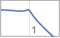
A third-order Chebyshev type 1 filter model:
tf = Chebyshev1FilterModel[3]Express the filter model in terms of variable ![]() :
:
tf = Chebyshev1FilterModel[3, s]Bode magnitude plot of the modeled filter:
BodePlot[tf, GridLines -> Automatic, PlotLayout -> "Magnitude"]A lowpass Chebyshev type 1 filter using the full specification:
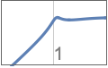
tf = Chebyshev1FilterModel[{"Lowpass", {1., 2.}, {1., 20.}}, s]//ChopMagnitude response of the filter showing the ideal filter characteristics:
Plot[Abs[tf[I * ω]], {ω, 0, 3}, PlotRange -> All, Epilog -> {Pink, Dashed, Line[{{0, 0.89}, {1, 0.89}, {1, 0.1}}], Line[{{2., 0.89}, {2., 0.1}, {3., 0.1}}]}]Scope (5)
Create a symbolic Chebyshev type 1 filter model of a lowpass filter:
Chebyshev1FilterModel[{2, ω}, s]//NExact computation of the model:
Chebyshev1FilterModel[{2, 1}, s]Computation of the model with precision 24:
Chebyshev1FilterModel[{2, N[1, 24]}, s]Create a highpass Chebyshev type 1 filter:
BodePlot[Chebyshev1FilterModel[{"Highpass", {1., 2.}, {20., 1.}}], GridLines -> Automatic, PlotLayout -> "Magnitude"]Create a bandpass filter with passband frequencies 1 and 10 and attenuation of order 3:
BodePlot[Chebyshev1FilterModel[{"Bandpass", 3, {1, 10}}], {0.1, 100}, GridLines -> Automatic, PlotLayout -> "Magnitude"]Use center frequency 1 and quality factor 1/3:
BodePlot[Chebyshev1FilterModel[{"Bandpass", 3, {{1, 1 / 3}}}], {0.01, 100}, GridLines -> Automatic, PlotLayout -> "Magnitude"]Create a bandpass Chebyshev type 1 filter using the full specification:
tf = Chebyshev1FilterModel[{"Bandpass", {0.1, 1., 10., 100.}, {60, -20Log10[1 / Sqrt[2]]}}];BodePlot[tf, {0.1, 100}, GridLines -> Automatic, PlotLayout -> "Magnitude"]Create a bandstop filter with passband frequencies 1 and 10 and attenuation of order 3:
BodePlot[Chebyshev1FilterModel[{"Bandstop", 3, {1, 10}}], {0.1, 100}, GridLines -> Automatic, PlotLayout -> "Magnitude"]Use center frequency 1 and quality factor 1/3:
BodePlot[Chebyshev1FilterModel[{"Bandstop", 3, {{1, 1 / 3}}}], {0.01, 100}, GridLines -> Automatic, PlotLayout -> "Magnitude"]Create a bandstop Chebyshev type 1 filter using the full specification:
tf = Chebyshev1FilterModel[{"Bandstop", {0.1, 1., 10., 100.}, {1, 20}}];
BodePlot[tf, {0.01, 1000.}, GridLines -> Automatic, PlotLayout -> "Magnitude"]
Applications (5)
Create a lowpass Chebyshev type 1 filter:
tf = Chebyshev1FilterModel[{"Lowpass", {1., 2.}, {1, 40}}];Filter out high-frequency noise from a sinusoidal signal:
ω = 1 / 5;input = (Sin[ω t] + 1 / 2 Sin[25ω t]) UnitStep[t];
response1 = OutputResponse[tf, input, {t, 0, 100}][[1]];
Chebyshev type 1 filter phase shifts the response by Arg[tf[ω ]], where ω is the frequency of the input sinusoid:
Plot[{input, response1}, {t, 20, 100}]delay = Arg[tf[I ω]] / ω//First//First;
Plot[Evaluate[Flatten[{input, response1 /. t -> (t - delay)}]], {t, 20, 100}]Create a highpass Chebyshev type 1 filter from the lowpass prototype:
tf2 = TransferFunctionTransform[1 / #&, tf];Filter out low-frequency sinusoid from the input:
Plot[Evaluate[Flatten[{input, OutputResponse[tf2, input, {t, 0, 100}]}]], {t, 20, 100}]Design a digital lowpass filter using the Chebyshev 1 approximation that satisfies the following passband and stopband frequencies and attenuations:
Subscript[ω, p] = 0.4π;Subscript[ω, s] = 0.6π;
Subscript[a, p] = 1;Subscript[a, s] = 20;
Obtain the equivalent analog frequencies assuming a sampling period of 1:
{Subscript[Ω, p] = 2 Tan[(0.4π/2)], Subscript[Ω, s] = 2 Tan[(0.6π/2)]}Compute the analog Chebyshev 1 transfer function:
tf = Chebyshev1FilterModel[{"Lowpass", {Subscript[Ω, p], Subscript[Ω, s]}, {Subscript[a, p], Subscript[a, s]}}, s]Convert to discrete-time model:
dtf = ToDiscreteTimeModel[tf, 1, z]//ChopBodePlot[dtf, {0.1 π, π}, PlotLayout -> "Magnitude", GridLines -> {{Subscript[ω, p], Subscript[ω, s]}, {10^-Subscript[a, p] / 20, 10^-Subscript[a, s] / 20}}, ScalingFunctions -> {"Linear", "Absolute"}, PlotRange -> All]Create a length 31 FIR approximation of the discrete-time Chebyshev 1 IIR filter:
OutputResponse[dtf, KroneckerDelta[n], {n, 0, 30}]//ChopListPlot[%, PlotRange -> All, Filling -> 0]Smooth financial data using an FIR approximation of a Chebyshev filter:
data = Transpose[FinancialData["GE", {"Jan. 1, 2012", "Jan. 1, 2013"}]["Path"]];
fir = OutputResponse[ToDiscreteTimeModel[Chebyshev1FilterModel[{3, 1.}], 1], KroneckerDelta[n], {n, 0, 40}]//Chop//Flatten;
DateListPlot[{Transpose[data], Transpose[{data[[1]], -ListConvolve[fir, data[[2]], 4]}]}, PlotRange -> All, PlotLegends -> {"original", "smoothed"}]
Filter an image using a discrete-time lowpass Chebyshev type 1 filter:
h = ToDiscreteTimeModel[Chebyshev1FilterModel[{"Lowpass", 3, 0.75}], 1];
RecurrenceFilter[h, [image]]
Filter an image using a highpass Chebyshev type 1 filter:
h = ToDiscreteTimeModel[Chebyshev1FilterModel[{"Highpass", 3, 0.75}], 1];
RecurrenceFilter[h, [image]]
Properties & Relations (8)
Stopband attenuation increases as order n increases:
tf = Chebyshev1FilterModel[{"Lowpass", #}]& /@ {1, 2, 3};
BodePlot[tf, {0.1, 10}, GridLines -> Automatic, PlotLayout -> "Magnitude", PlotLegends -> {1, 2, 3}]
Passband width of "Bandpass" filter decreases with increasing quality factor q:
tf = Chebyshev1FilterModel[{"Bandpass", 2, {{1, #}}}]& /@ {0.5, 1., 3.};
BodePlot[tf, {0.1, 10}, GridLines -> Automatic, PlotLayout -> "Magnitude", PlotRange -> {0, -80}, PlotLegends -> {0.5, 1., 3.}]
Phase response of a third-order "Lowpass" type 1 Chebyshev filter:
BodePlot[Chebyshev1FilterModel[{"Lowpass", 3}], {0.1, 10.}, PlotLayout -> "Phase", GridLines -> Automatic]Compare phase responses for different filter orders:
BodePlot[Chebyshev1FilterModel[{"Lowpass", #}]& /@ {1, 2, 3}, {0.1, 10.}, PlotLayout -> "Phase", GridLines -> Automatic, PlotLegends -> {1, 2, 3}]Phase response of a "Bandpass" filter for several quality factors:
BodePlot[Chebyshev1FilterModel[{"Bandpass", 2, {{1, #}}}]& /@ {1., 3., 5.}, {0.1, 10}, GridLines -> Automatic, PlotLayout -> "Phase", PlotLegends -> {1., 3., 5.}]Compare Chebyshev type 1 and type 2 lowpass filters:
t1 = Chebyshev1FilterModel[{"Lowpass", {1., 2.}, {1., 20.}}, s]t2 = Chebyshev2FilterModel[{"Lowpass", {1., 2.}, {1., 20.}}, s]Plot[{Abs[t1[I * ω]], Abs[t2[I * ω]]}, {ω, 0, 3}, PlotRange -> All, Epilog -> {Pink, Dashed, Line[{{0, 0.89}, {1, 0.89}, {1, 0.1}}], Line[{{2., 0.89}, {2., 0.1}, {3., 0.1}}]}]Extract the order of the Chebyshev type 1 polynomial:
SystemsModelOrder[StateSpaceModel[Chebyshev1FilterModel[{"Lowpass", {1., 2.}, {1., 20.}}]]]Find the poles of a Chebyshev type 1 filter:
tfm = Chebyshev1FilterModel[11];
poles = TransferFunctionPoles[tfm]
Plot poles of the Butterworth filter:
PoleZeroPlot[tfm, ...]Implement a lowpass digital Chebyshev type 1 filter:
dtfm = ToDiscreteTimeModel[Chebyshev1FilterModel[11], 1]Plot poles of the digital Chebyshev type 1 filter:
PoleZeroPlot[dtfm]Convert a lowpass filter to highpass:
lo = Chebyshev1FilterModel[3];
hi = TransferFunctionTransform[(1 / #&), lo];BodePlot[{lo, hi}, {0.1, 10}, GridLines -> Automatic, PlotLayout -> "Magnitude"]Text
Wolfram Research (2012), Chebyshev1FilterModel, Wolfram Language function, https://reference.wolfram.com/language/ref/Chebyshev1FilterModel.html (updated 2016).
CMS
Wolfram Language. 2012. "Chebyshev1FilterModel." Wolfram Language & System Documentation Center. Wolfram Research. Last Modified 2016. https://reference.wolfram.com/language/ref/Chebyshev1FilterModel.html.
APA
Wolfram Language. (2012). Chebyshev1FilterModel. Wolfram Language & System Documentation Center. Retrieved from https://reference.wolfram.com/language/ref/Chebyshev1FilterModel.html