Wolfram Language & System Documentation Center

DiffusionPDETerm

DiffusionPDETerm[vars]

represents a diffusion term with model variables vars.

DiffusionPDETerm[vars,c]

represents a diffusion term with diffusion coefficient .

DiffusionPDETerm[vars,c,pars]

uses model parameters pars.

Details

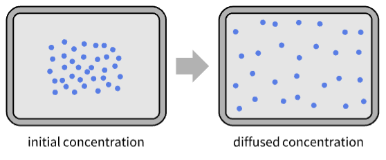
Diffusion is a central concept of physics that is used in a number of domains, such as thermodynamics, acoustics, structural mechanics and fluid dynamics.
Diffusion is also known as conduction.
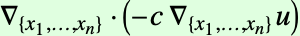
Diffusion with a diffusion coefficient is the process of equilibration solely driven by a gradient of the dependent variable :

DiffusionPDETerm returns a differential operators term to be used as a part of partial differential equations:

DiffusionPDETerm can be used to model diffusion equations with dependent variable , independent variables and time variable .
Stationary model variables vars are vars={u[x₁,…,x_n],{x₁,…,x_n}}.
Time-dependent model variables vars are vars={u[t,x₁,…,x_n],{x₁,…,x_n}} or vars={u[t,x₁,…,x_n],t,{x₁,…,x_n}}.
The diffusion term in context with other PDE terms is given by:

During diffusion, the medium in which the diffusion happens remains stationary, in contrast to convection where the medium is the transport mechanism.
The diffusion coefficient can have the following forms:

			scalar , isotropic diffusion
	{c₁,…,c_n}		vector , orthotropic diffusion
	{{c₁₁,…,c_1n},…,{c_n1,…,c_nn}}		matrix , anistropic diffusion

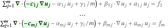
For a system of PDEs with dependent variables {u₁,…,u_m}, the diffusion represents:

The diffusion term in context systems of PDE terms:

The diffusion coefficient is a tensor of rank 4 of the form where each submatrix is an matrix that can be specified in the same way as for a single dependent variable.
A symbolic diffusion coefficient can be specified through a MatrixSymbol. »
The diffusion coefficient can depend on time, space, parameters and the dependent variables.
The following parameters pars can be given:
parameter default symbol

"CoordinateChart" "Cartesian"

"RegionSymmetry" None
A possible choice for the parameter "RegionSymmetry" is "Axisymmetric".
"Axisymmetric" region symmetry represents a truncated cylindrical coordinate system where the cylindrical coordinates are reduced by removing the angle variable as follows:
dimension reduction equation

1D

2D
The coefficient affects the meaning of NeumannValue.
All quantities that do not explicitly depend on the independent variables given are taken to have zero partial derivative.

Examples

open all close all

Basic Examples (6)

Define a stationary diffusion term:

Wolfram Language code: DiffusionPDETerm[{u[x], {x}}, 1]

Activate the term:

Wolfram Language code: Activate[%]

Define a stationary diffusion term with a parametric diffusion coefficient replaced:

Wolfram Language code: DiffusionPDETerm[{u[x], {x}}, κ, <|κ -> 1|>]

Activate the term:

Wolfram Language code: Activate[%]

Define a symbolic diffusion term:

Wolfram Language code: DiffusionPDETerm[{u[x], {x}}, {{κ[x]}}]

Activate the term:

Wolfram Language code: Activate[%]

Find the eigenvalues of a diffusion term:

Wolfram Language code: NDEigenvalues[DiffusionPDETerm[{u[x], {x}}], u, {x}∈Line[{{0}, {1}}], 3]

Construct a Poisson equation from basic terms and solve it symbolically:

Wolfram Language code:

vars = {u[x, y], {x, y}};
DSolveValue[Activate[DiffusionPDETerm[vars] == SourcePDETerm[vars, 1]], u[x, y], {x, y}]

Solve a time-dependent diffusion equation with a Gaussian initial condition:

Wolfram Language code:

ufun = NDSolveValue[{D[u[t, x], t] + DiffusionPDETerm[{u[t, x], {x}}, 1] == 0, u[0, x] == Exp[-x ^ 2]}, u, {t, 0, 1}, {x, -π, π}]

Visualize the smoothing of the initial condition through time:

Wolfram Language code: Plot[Evaluate[Table[ufun[t, x], {t, 0, 1, 0.25}]], {x, -π, π}, Rule[...]]

Check that the area under the curves remains constant:

Wolfram Language code: NIntegrate[ufun[0, x], {x, -π, π}] - NIntegrate[ufun[1, x], {x, -π, π}]

Scope (36)

1D (6)

Define a symbolic matrix diffusion term:

Wolfram Language code: DiffusionPDETerm[{u[t, x], {x}}, MatrixSymbol["c", {1, 1}]]

Activate the term:

Wolfram Language code: Activate[%]

Not specifying a diffusion coefficient will result in an identity matrix coefficient:

Wolfram Language code: DiffusionPDETerm[{u[x], {x}}]

Define a time-dependent diffusion term:

Wolfram Language code: DiffusionPDETerm[{u[t, x], {x}}, {{1 + t}}]

Activate the term:

Wolfram Language code: Activate[%]

Define a stationary diffusion term with a parametric diffusion coefficient replaced:

Wolfram Language code:

κ = MatrixSymbol["c", {1, 1}];
DiffusionPDETerm[{u[x], {x}}, κ, <|{κ -> {{1}}}|>]

Activate the term:

Wolfram Language code: Activate[%]

Use DiffusionPDETerm for modeling an eigenvalue problem:

Wolfram Language code: NDEigensystem[DiffusionPDETerm[{u[x], {x}}, 1], u, {x, 0, 1}, 3]

Use DiffusionPDETerm to set up a 1D Poisson equation:

Wolfram Language code: NDSolveValue[{DiffusionPDETerm[{u[x], {x}}, 1] == 1, DirichletCondition[u[x] == 0, True]}, u, {x, 0, 1}]

Visualize the result:

Wolfram Language code: Plot[%[x], {x, 0, 1}]

1D Axisymmetric (1)

Set up a 1D axisymmetric diffusion equation:

Wolfram Language code: DiffusionPDETerm[{u[r], {r}}, 1, <|"RegionSymmetry" -> "Axisymmetric"|>]

Apply Activate to the term:

Wolfram Language code: Activate[%]

Verify that the axisymmetric case is a consequence of using a truncated cylindrical coordinate system using the operators that compose the diffusion equation:

Wolfram Language code: Div[-1 * Grad[u[r], {r, θ, z}, "Cylindrical"], {r, θ, z}, "Cylindrical"]

2D (13)

Define a 2D stationary diffusion term:

Wolfram Language code: DiffusionPDETerm[{u[x, y], {x, y}}, 1]

Activate the term:

Wolfram Language code: Activate[%]

Not specifying a diffusion coefficient will result in an identity matrix coefficient:

Wolfram Language code: DiffusionPDETerm[{u[x, y], {x, y}}]

Set up a 2D stationary diffusion equation:

Wolfram Language code: DiffusionPDETerm[{u[x, y], {x, y}}, 1] == 0

Activate the term:

Wolfram Language code: Activate[%]

Define a symbolic matrix diffusion term:

Wolfram Language code: DiffusionPDETerm[{u[x, y], {x, y}}, MatrixSymbol["c", {2, 2}]]

Activate the term:

Wolfram Language code: Activate[%]

Set up a 2D time-dependent diffusion equation:

Wolfram Language code: D[u[t, x, y]] + DiffusionPDETerm[{u[t, x, y], {x, y}}, 1] == 0

Activate the term:

Wolfram Language code: Activate[%]

Define a 2D orthotropic stationary diffusion term with a vector diffusion coefficient:

Wolfram Language code: DiffusionPDETerm[{u[x, y], {x, y}}, {10, 20}]

Define a 2D stationary diffusion term with an anisotropic diffusion matrix:

Wolfram Language code: DiffusionPDETerm[{u[x, y], {x, y}}, {{2, 1}, {0, 1}}]

Define a 2D diffusion term with an anisotropic diffusion matrix:

Wolfram Language code: DiffusionPDETerm[{u[t, x, y], t, {x, y}}, {{2, 1}, {0, 1}}]

Use DiffusionPDETerm to set up a 2D Poisson equation:

Wolfram Language code:

NDSolveValue[{DiffusionPDETerm[{u[x, y], {x, y}}, 1] == 1, DirichletCondition[u[x, y] == 0, True]}, u, {x, y}∈Rectangle[]]

Visualize the result:

Wolfram Language code: ContourPlot[%[x, y], {x, y}∈Rectangle[]]

Construct a Poisson equation from basic PDE terms and solve it numerically:

Wolfram Language code:

vars = {u[x, y], {x, y}};
NDSolveValue[{DiffusionPDETerm[vars] == SourcePDETerm[vars, 1], DirichletCondition[u[x, y] == 0, True]}, u[x, y], {x, y}∈Disk[]]

Visualize the result:

Wolfram Language code: Plot3D[%, {x, y}∈Disk[]]

Use a vector-valued diffusion coefficient that has a larger diffusion constant in the direction than the direction:

Wolfram Language code:

NDSolveValue[{DiffusionPDETerm[{u[x, y], {x, y}}, {10, 1}] == 1, DirichletCondition[u[x, y] == 0, True]}, u, {x, y}∈Rectangle[]]

Visualize the result:

Wolfram Language code: ContourPlot[%[x, y], {x, y}∈Rectangle[]]

Use a vector-valued diffusion coefficient that has a larger diffusion constant in the direction than the direction:

Wolfram Language code:

NDSolveValue[{DiffusionPDETerm[{u[x, y], {x, y}}, {1, 10}] == 1, DirichletCondition[u[x, y] == 0, True]}, u, {x, y}∈Rectangle[]]

Visualize the result:

Wolfram Language code: ContourPlot[%[x, y], {x, y}∈Rectangle[]]

Use an anisotropic diffusion coefficient:

Wolfram Language code:

NDSolveValue[{DiffusionPDETerm[{u[x, y], {x, y}}, {{1, 1 / 2}, {1 / 2, 1}}] == 1, DirichletCondition[u[x, y] == 0, True]}, u, {x, y}∈Rectangle[]]

Visualize the result:

Wolfram Language code: ContourPlot[%[x, y], {x, y}∈Rectangle[]]

2D Axisymmetric (3)

Set up a 2D axisymmetric diffusion equation:

Wolfram Language code: DiffusionPDETerm[{u[r, z], {r, z}}, 1, <|"RegionSymmetry" -> "Axisymmetric"|>] == 0

Apply Activate to the term:

Wolfram Language code: Activate[%]

Verify that the axisymmetric case is a consequence of using a truncated cylindrical coordinate system using the operators that compose the diffusion equation:

Wolfram Language code: Div[{{-1, 0, 0}, {0, -1, 0}, {0, 0, -1}}. Grad[u[r, z], {r, θ, z}, "Cylindrical"], {r, θ, z}, "Cylindrical"]

Set up a 2D axisymmetric diffusion equation:

Wolfram Language code: DiffusionPDETerm[{u[r, z], {r, θ, z}}, 1, <|"RegionSymmetry" -> "Axisymmetric"|>]

Apply Activate to the term:

Wolfram Language code: Activate[%]

Set up a 2D axisymmetric time-dependent diffusion equation:

Wolfram Language code: D[u[t, r, z]] + DiffusionPDETerm[{u[t, r, z], {r, z}}, 1, <|"RegionSymmetry" -> "Axisymmetric"|>] == 0

Apply Activate to the term:

Wolfram Language code: Activate[%]

3D (1)

Use DiffusionPDETerm to set up a 3D Poisson equation:

Wolfram Language code:

usol  = NDSolveValue[
	{DiffusionPDETerm[{u[x, y, z], {x, y, z}}, -1] == 1, 
	DirichletCondition[u[x, y, z] == x y z, True]}, u, {x, y, z}∈ Ball[]]

Visualize the result:

Wolfram Language code: DensityPlot3D[usol[x, y, z], {x, y, z}∈Ball[], PlotLegends -> Automatic, AxesLabel -> Automatic]

Coordinate Chart (3)

Define a diffusion term with a coordinate chart:

Wolfram Language code: DiffusionPDETerm[{u[r, z], {r, z}}, 1, <|"CoordinateChart" -> "Polar"|>]

Activate the operator:

Wolfram Language code: Activate[%]

Compare with a Laplacian:

Wolfram Language code: Laplacian[u[r, z], {r, z}, "Polar"]

Find eigenvalues and vectors of a diffusion term in polar coordinates:

Wolfram Language code:

{vals, funs} = NDEigensystem[{DiffusionPDETerm[{u[r, θ], {r, θ}}, 1, <|"CoordinateChart" -> "Polar"|>], DirichletCondition[u[r, θ] == 0, r == π], PeriodicBoundaryCondition[u[r, θ], θ == -π && r < π, Function[X, X + {0, 2π}]]}, u, {r, θ}∈Rectangle[{0, -π}, {π, π}], 4]

Visualize eigenvectors of a Laplacian term in polar coordinates:

Wolfram Language code: RevolutionPlot3D[#[r, θ], {r, 0, π}, {θ, -π, π}, PlotRange -> All]& /@ funs

Solve a PDE in polar coordinates:

Wolfram Language code:

ifun = NDSolveValue[{DiffusionPDETerm[{u[r, θ], {r, θ}}, 1, <|"CoordinateChart" -> "Polar"|>] == 0, DirichletCondition[u[r, θ] == Sin[4 θ], r == π], DirichletCondition[u[r, θ] == 0, θ == -π || θ == π]}, u, {r, θ}∈Rectangle[{0, -π}, {π, π}]]

Plot the solution in Cartesian coordinates:

Wolfram Language code: Plot3D[Evaluate[ifun[r, θ] /. {r -> Sqrt[x ^ 2 + y ^ 2], θ -> ArcTan[x, y]}], {x, y}∈Disk[{0, 0}, π]]

Coupled (6)

Define a diffusion term with multiple dependent variables:

Wolfram Language code: DiffusionPDETerm[{{u[x], v[x]}, {x}}]

Define a diffusion term with multiple dependent variables:

Wolfram Language code: DiffusionPDETerm[{{u[x], v[x]}, {x}}, 1]

Define a diffusion term with multiple dependent variables and multiple diffusion coefficients:

Wolfram Language code: DiffusionPDETerm[{{u[x], v[x]}, {x}}, {{Subscript[c, 11], Subscript[c, 12]}, {Subscript[c, 21], Subscript[c, 22]}}]

Define a diffusion term with multiple dependent variables and anisotropic diffusion coefficients:

Wolfram Language code:

DiffusionPDETerm[{{u[x, y], v[x, y]}, {x, y}}, {{Subscript[c, 11], {Subscript[c, 1211], Subscript[c, 1222]}}, {0, {{Subscript[c, 2211], Subscript[c, 2212]}, {Subscript[c, 2221], Subscript[c, 2222]}}}}]

Define a diffusion term with multiple dependent variables and all coefficients specified:

Wolfram Language code: cIn = Array[Subscript[c, ##]&, {2, 2, 2, 2}]

Wolfram Language code: DiffusionPDETerm[{{u[x, y], v[x, y]}, {x, y}}, cIn]

Off-diagonal diffusion coefficients are possible in coupled PDEs:

Wolfram Language code: MatrixForm[coefficients = {{{{1, 0}, {0, 1}}, {{0, 2}, {2, 0}}}, {{{0, 0}, {0, 0}}, {{1, 0}, {0, 1}}}}]

Solve the equations:

Wolfram Language code:

{uif, vif} = NDSolveValue[{DiffusionPDETerm[{{u[x, y], v[x, y]}, {x, y}}, coefficients] == {1, 1}, DirichletCondition[{u[x, y] == 0, v[x, y] == 0}, True]}, {u, v}, {x, y}∈Rectangle[]];

Visualize the results:

Wolfram Language code: GraphicsRow[{ContourPlot[uif[x, y], {x, y}∈Rectangle[]], ContourPlot[vif[x, y], {x, y}∈Rectangle[]]}]

Coupled Axisymmetric (3)

Use DiffusionPDETerm to set up a 1D axisymmetric equation with multiple dependent variables:

Wolfram Language code: eqn = DiffusionPDETerm[{{u[r], v[r]}, {r}}, {{2.4, 3}, {3, 3}}, <|"RegionSymmetry" -> "Axisymmetric"|>] == {1, 1}

Specify boundary conditions:

Wolfram Language code: bcs = {u[0.1] == 200, v[0.1] == 200, u[0.5] == 50, v[0.5] == 5};

Solve the equations numerically:

Wolfram Language code: {uif, vif} = NDSolveValue[{eqn, bcs}, {u, v}, {r, 0.1, 0.5}]

Solve the same equation symbolically:

Wolfram Language code: {fufun, fvfun} = DSolveValue[{eqn, bcs}, {u, v}, {r}]

Visualize the difference between the results:

Wolfram Language code: Plot[{fufun[r] - uif[r], fvfun[r] - vif[r]}, {r, 0.1, 0.5}, PlotLegends -> "Expressions", PlotRange -> All]

Define an axisymmetric diffusion term with multiple dependent variables:

Wolfram Language code: DiffusionPDETerm[{{u[r, z], v[r, z]}, {r, z}}, 1, <|"RegionSymmetry" -> "Axisymmetric"|>]

Apply Activate to the term:

Wolfram Language code: Activate[%]

Define a 2D diffusion axisymmetric term with multiple dependent variables and multiple diffusion coefficients:

Wolfram Language code:

MatrixForm[
	coefficients = {{{{25, 0}, {0, 25}}, {{0, 10}, {5, 0}}}, {{{0, 15}, {20, 0}}, {{50, 0}, {0, 25}}}}]

Wolfram Language code: coupledPDEs = DiffusionPDETerm[{{u[r, z], v[r, z]}, {r, z}}, coefficients, <|"RegionSymmetry" -> "Axisymmetric"|>];

Solve the coupled PDEs:

Wolfram Language code:

{uif, vif} = NDSolveValue[{coupledPDEs == {1, 1}, DirichletCondition[{u[r, z] == 0, v[r, z] == 0}, z == 0]}, {u, v}, {r, z}∈Rectangle[]];

Visualize the results:

Wolfram Language code: GraphicsRow[{ContourPlot[uif[r, z], {r, z}∈Rectangle[]], ContourPlot[vif[r, z], {r, z}∈Rectangle[]]}]

Applications (9)

Use DiffusionPDETerm with a variable diffusion coefficient:

Wolfram Language code: model = DiffusionPDETerm[{u[x], {x}}, {{If[x ≤ 3 / 4, 1, 2]}}]

Solve the equation:

Wolfram Language code:

solution = NDSolveValue[{model == 0, DirichletCondition[u[x] == 1, x == 0], DirichletCondition[u[x] == 0, x == 1]}, u, {x, 0, 1}]

Compute the flux:

Wolfram Language code: flux = model /. Inactive[Div][flux_, _] :> Activate[flux]

Visualize the result:

Wolfram Language code: Plot[Evaluate[{solution[x], flux /. u -> solution}], {x, 0, 1}, ...]

Use DiffusionPDETerm to model conductive heat transfer using an axisymmetric geometry.

The region of analysis is a 2D region. Instead of defining the full 2D region in Cartesian coordinates , you can define a region with truncated cylindrical coordinates in 1D . The cylindrical coordinate variables and vanish because the system is rotationally symmetric around the axis.

Set up the equation:

Wolfram Language code: eqn = DiffusionPDETerm[{u[r], {r}}, 2.4, <|"RegionSymmetry" -> "Axisymmetric"|>] == 0

Specify boundary conditions:

Wolfram Language code: bcs = {u[1 / 10] == 200, u[1 / 2] == 50};

Solve the equation:

Wolfram Language code: numericSolution = NDSolveValue[{eqn, bcs}, u, {r, 0.1, 0.5}]

Or solve it symbolically with DSolveValue:

Wolfram Language code: analytocalSolution = DSolveValue[{eqn, bcs}, u, r]

Visualize the difference between the results:

Wolfram Language code: Plot[analytocalSolution[r] - numericSolution[r], {r, 0.1, 0.5}, PlotRange -> All]

Use DiffusionPDETerm to model species diffusion under a dam. Set up the region:

Wolfram Language code:

Subscript[Ω, dam] = Rectangle[{6, 3}, {12, 18}];
Subscript[Ω, sediment] = RegionDifference[Rectangle[{0, 0}, {18, 6}], Subscript[Ω, dam]];

Set up the model:

Wolfram Language code: model = DiffusionPDETerm[{u[x, y], {x, y}}, 10 ^ -4]

Solve the equation:

Wolfram Language code:

solution = NDSolveValue[{model == 0, DirichletCondition[u[x, y] == 16, x ≤ 6 && y == 6], DirichletCondition[u[x, y] == 8, x ≥ 12 && y == 6]}, u, {x, y}∈Subscript[Ω, sediment]]

Compute the flux:

Wolfram Language code: flux = model /. Inactive[Div][flux_, _] :> Activate[flux]

Visualize the result:

Wolfram Language code:

Show[
	..., 
	VectorPlot[Evaluate[flux /. u -> solution], {x, y}∈Subscript[Ω, sediment], Rule[...]]]

Find the concentration of species under the dam. Construct the model:

Wolfram Language code:

op = DiffusionPDETerm[{c[x, y], {x, y}}, 1] + ConvectionPDETerm[{c[x, y], {x, y}}, flux /. u -> solution] + 2 * 10 ^ -5c[x, y];

Solve the equation:

Wolfram Language code:

concentration = NDSolveValue[{op == 0, 
	DirichletCondition[c[x, y] == 100, x ≤ 6 && y == 6], DirichletCondition[c[x, y] == 50, x ≥ 12 && y == 6]
	}, c, {x, y}∈Subscript[Ω, sediment]]

Visualize the species concentration:

Wolfram Language code:

Show[
	..., 
	ContourPlot[concentration[x, y], {x, y}∈Subscript[Ω, sediment], ...], 
	VectorPlot[Evaluate[flux /. u -> solution], {x, y}∈Subscript[Ω, sediment], Rule[...]]
	]

Define a Helmholtz model:

Wolfram Language code: helmholtzModel[vars_, k_] := DiffusionPDETerm[vars, 1] + ReactionPDETerm[vars, k]

Solve for the eigenvalues of the Helmholtz equation:

Wolfram Language code: NDEigenvalues[{helmholtzModel[{u[x, y], {x, y}}, 4]}, u, {x, y}∈Disk[], 5]

Solve the Helmholtz equation with a source term:

Wolfram Language code:

vars = {u[x, y], {x, y}};
NDSolveValue[{helmholtzModel[vars, 4] == SourcePDETerm[vars, 1], DirichletCondition[u[x, y] == 0, True]}, u[x, y], {x, y}∈Disk[]]

Visualize the solution:

Wolfram Language code: Plot3D[%, {x, y}∈Disk[]]

Use DiffusionPDETerm to model conductive heat transfer using an axisymmetric geometry. The region of analysis is a 3D hollow cylinder. Instead of defining the full 3D region in Cartesian coordinates , you can define a region with truncated cylindrical coordinates in 2D . The cylindrical coordinate variable vanishes because the system is rotationally symmetric around the axis.

Set up the region:

Wolfram Language code: Ω = Rectangle[{0.02, 0}, {0.1, 0.14}];

Set up the PDE model:

Wolfram Language code: model = DiffusionPDETerm[{u[r, z], {r, z}}, 52, <|"RegionSymmetry" -> "Axisymmetric"|>]

Solve the axisymmetric equation:

Wolfram Language code:

solution = NDSolveValue[{model == NeumannValue[5 * 10 ^ 5, r == 0.02  && (0.04 <= z <= 0.1)], DirichletCondition[u[r, z] == 273.15, z == 0 || r == 0.1 || z == 0.14]}, u, {r, z}∈Ω]

Visualize the result:

Wolfram Language code: ContourPlot[solution[r, z], {r, z}∈Ω, ...]

Visualize the result in 3D space for part of the cylinder:

Wolfram Language code:

Legended[RegionPlot3D[0.02^2 ≤ x^2 + y^2 ≤ 0.1^2 && 0 ≤ PlanarAngle[{0, 0} -> {{0.02, 0}, {x, y}}] ≤ (4 π/3), {x, -0.1, 0.1}, {y, -0.1, 0.1}, {z, 0, 0.14}, ...], BarLegend[...]]

Use DiffusionPDETerm to model a nonlinear conductive heat transfer using an axisymmetric geometry.

Set up the region:

Wolfram Language code:

radius = 3;
height = 8;
Ω2D = Rectangle[{0, 0}, {radius, height}];

Find the thermal conductivity for air:

Wolfram Language code: Subscript[k, air] = QuantityMagnitude[ThermodynamicData["Air", "ThermalConductivity"]];

Set up the PDE model:

Wolfram Language code:

flux = 10;
temperature = 10;
model2D = {DiffusionPDETerm[{u[r, z], {r, z}}, (Subscript[k, air] + 10^-3u[r, z]) * IdentityMatrix[2], <|"RegionSymmetry" -> "Axisymmetric"|>] == NeumannValue[flux, r == radius], DirichletCondition[u[r, z] == temperature, z == 0]};

Solve the equation and measure the time and memory needed to do so:

Wolfram Language code:

measure2D  = 
	AbsoluteTiming[
	MaxMemoryUsed[
	solution2D = NDSolveValue[model2D, u, {r, z}∈Ω2D]]];

Visualize the axisymmetric result:

Wolfram Language code: ContourPlot[solution2D[r, z], {r, z}∈Ω2D, ...]

Print the total time to do the computation and number of megabytes used during the evaluation:

Wolfram Language code:

Print["Time -> ", measure2D[[1]], " s", "
Memory -> ", measure2D[[2]] / (1024. ^ 2), " MB"]

Use DiffusionPDETerm to set up a plane stress operator. Set up the coupled coefficients:

Wolfram Language code:

MatrixForm[coefficients = {{{{(Y/1 - ν^2), 0}, {0, (Y (1 - ν)/2 (1 - ν^2))}}, {{0, (Y ν/1 - ν^2)}, {(Y (1 - ν)/2 (1 - ν^2)), 0}}}, {{{0, (Y (1 - ν)/2 (1 - ν^2))}, {(Y ν/1 - ν^2), 0}}, {{(Y (1 - ν)/2 (1 - ν^2)), 0}, {0, (Y/1 - ν^2)}}}}]

Set up the model:

Wolfram Language code: model = DiffusionPDETerm[{{u[x, y], v[x, y]}, {x, y}}, coefficients, <|ν -> 1 / 3, Y -> 10 ^ 3|>]

Set up a region:

Wolfram Language code: Ω = Rectangle[{0, 0}, {5, 1}]

Solve the equations:

Wolfram Language code:

{uif, vif} = NDSolveValue[{model == {0, NeumannValue[-1, x == 5]}, DirichletCondition[{u[x, y] == 0., v[x, y] == 0.}, x == 0]}, {u, v}, {x, y}∈Ω]

Visualize the results:

Wolfram Language code: ContourPlot[uif[x, y], {x, y}∈Ω, ...]

Wolfram Language code: ContourPlot[vif[x, y], {x, y}∈Ω, ...]

Compute the flux:

Wolfram Language code: flux = model /. Inactive[Div][flux_, _] :> Activate[flux]

Define a Stokes-flow model:

Wolfram Language code:

stokesModel[vars_, μ_] := DiffusionPDETerm[vars, {{μ, 0, 0}, {0, μ, 0}, {0, 0, 0}}] + ConvectionPDETerm[vars, {{0, 0, {1, 0}}, {0, 0, {0, 1}}, {{1, 0}, {0, 1}, 0}}]

Set up the equation:

Wolfram Language code: eqn = stokesModel[{{u[x, y], v[x, y], p[x, y]}, {x, y}}, 1] == {0, 0, 0}

Define a narrowing region:

Wolfram Language code: Ω = RegionUnion[Rectangle[{0, 0}, {1, 1 / 2}], Rectangle[{1, 1 / 10}, {2, 2 / 5}]];

Set up a boundary condition:

Wolfram Language code:

bcs = {DirichletCondition[
	{u[x, y] == 4 * 0.3 * y * (0.5 - y) / (0.41) ^ 2, v[x, y] == 0.}, x == 0.], DirichletCondition[{u[x, y] == 0., v[x, y] == 0.}, 0 < x < 2], 
	DirichletCondition[p[x, y] == 0., x == 2]};

Solve the equation:

Wolfram Language code:

{xVel, yVel, pressure} = NDSolveValue[{eqn, bcs}, {u, v, p}, {x, y}∈Ω, Method -> {"FiniteElement", "InterpolationOrder" -> {u -> 2, v -> 2, p -> 1}, "MeshOptions" -> {"MaxCellMeasure" -> 0.0005}}];

Visualize the solution:

Wolfram Language code:

VectorPlot[{xVel[x, y], yVel[x, y]}, {x, y}∈Ω, AspectRatio -> Automatic, StreamPoints -> 6, StreamColorFunction -> "TemperatureMap", StreamColorFunctionScaling -> False]//Quiet

Extend a Stokes-flow model to a Navier–Stokes-flow model. Define a Stokes-flow model:

Wolfram Language code:

stokesModel[vars_, μ_] := DiffusionPDETerm[vars, {{μ, 0, 0}, {0, μ, 0}, {0, 0, 0}}] + ConvectionPDETerm[vars, {{0, 0, {1, 0}}, {0, 0, {0, 1}}, {{1, 0}, {0, 1}, 0}}]

Define a Navier–Stokes-flow model:

Wolfram Language code:

navierStokesModel[vars_, μ_, ρ_] := stokesModel[vars, μ] + ConvectionPDETerm[vars, {{ρ vars[[1, {1, 2}]], 0, 0}, {0, ρ vars[[1, {1, 2}]], 0}, {0, 0, 0}}]

Set up the equation:

Wolfram Language code: eqn = navierStokesModel[{{u[x, y], v[x, y], p[x, y]}, {x, y}}, 1, 10 ^ -3] == {0, 0, 0}

Define a region:

Wolfram Language code: Ω = Rectangle[{0, 0}, {1, 1}];

Set up a boundary condition:

Wolfram Language code:

bcs = {DirichletCondition[
	{u[x, y] == 1, v[x, y] == 0}, y == 1], DirichletCondition[{u[x, y] == 0, v[x, y] == 0}, y < 1], 
	DirichletCondition[p[x, y] == 0, x == 0 && y == 1]};

Solve the equation:

Wolfram Language code:

{xVel, yVel, pressure} = NDSolveValue[{eqn, bcs}, {u, v, p}, {x, y}∈Ω, Method -> {"FiniteElement", "InterpolationOrder" -> {u -> 2, v -> 2, p -> 1}, "MeshOptions" -> {"MaxCellMeasure" -> 0.0005}}];

Visualize the solution:

Wolfram Language code:

VectorPlot[{xVel[x, y], yVel[x, y]}, {x, y}∈Ω, AspectRatio -> Automatic, StreamPoints -> 6, StreamColorFunction -> "TemperatureMap", StreamColorFunctionScaling -> False]//Quiet

Properties & Relations (3)

Verify that anisotropic diffusion is the same as :

Wolfram Language code:

sol1 = NDSolveValue[{DiffusionPDETerm[{u[x, y], {x, y}}, {{1, 1 / 2}, {0, 1}}] == 1, DirichletCondition[u[x, y] == 0, True]}, u, {x, y}∈Rectangle[]]

Wolfram Language code:

sol2 = NDSolveValue[{DiffusionPDETerm[{u[x, y], {x, y}}, {{1, 1 / 4}, {1 / 4, 1}}] == 1, DirichletCondition[u[x, y] == 0, True]}, u, {x, y}∈Rectangle[]]

Visualize that there is no difference in the two solutions:

Wolfram Language code: Plot3D[Chop[sol1[x, y] - sol2[x, y]], {x, y}∈Rectangle[]]

Solve a time-dependent diffusion equation with a Gaussian initial condition:

Wolfram Language code:

nfun = NDSolveValue[{D[u[t, x], t] + DiffusionPDETerm[{u[t, x], {x}}, 1] == 0, DirichletCondition[u[t, x] == 0, True], u[0, x] == Exp[-x ^ 2]}, u[t, x], {t, 0, 1}, {x, -π, π}]

The analytical solution is an infinite series:

Wolfram Language code:

afun = DSolveValue[{Activate[D[u[t, x], t] + DiffusionPDETerm[{u[t, x], {x}}, 1] == 0], u[t, -π] == 0, u[t, π] == 0, u[0, x] == Exp[-x ^ 2]}, u, {t, 0, 1}, {x, -π, π}]

Extract a few terms from the Inactive sum:

Wolfram Language code: asol = afun[t, x] /. {∞ -> 15}//Activate;

Visualize the difference between the numerical and the analytical solutions:

Wolfram Language code: Plot3D[asol - nfun, {x, -π, π}, {t, 0, 1}, AxesLabel -> {"x", "t"}, PlotRange -> All]

The equilibration property of the diffusion term manifests itself in the smoothing of a discontinuous initial condition:

Wolfram Language code:

ufun = NDSolveValue[{D[u[t, x], t] + DiffusionPDETerm[{u[t, x], {x}}, 1] == 0, DirichletCondition[u[t, x] == 0, True], u[0, x] == 1 / 2 - Abs[x - 1 / 2]}, u, {t, 0, 0.001}, x∈Line[{{0}, {1}}]]

Visualize the discontinuous initial condition and the smoothed evolution of the initial condition:

Wolfram Language code: Plot[{(1 / 2 - Abs[x - 1 / 2]), ufun[0.001, x]}, {x, 0, 1}, PlotRange -> {{0.35, 0.65}, {0.4, 0.51}}]

Possible Issues (3)

The negative sign in the operator does not need to be given:

Wolfram Language code: DiffusionPDETerm[{u[x], {x}}, c]

A symbolic diffusion coefficient is interpreted as a scalar coefficient in the following input:

Wolfram Language code: DiffusionPDETerm[{u[x], {x}}, c]

A subsequent substitution must account for that:

Wolfram Language code: DiffusionPDETerm[{u[x], {x}}, c, <|c -> 1|>]

Activate the term:

Wolfram Language code: DiffusionPDETerm[{u[x], {x}}, c]//Activate

A numeric diffusion coefficient will automatically be multiplied with an IdentityMatrix of proper dimensions:

Wolfram Language code: DiffusionPDETerm[{u[x], {x}}, 1]

A way to specify a symbolic matrix diffusion coefficient is through a MatrixSymbol:

Wolfram Language code:

cs = MatrixSymbol["c", {1, 1}];
DiffusionPDETerm[{u[x], {x}}, cs, <|cs -> {{1}}|>]

Using a MatrixSymbol allows for activation of the operator:

Wolfram Language code: DiffusionPDETerm[{u[x], {x}}, cs]//Activate

DiffusionPDETerm models , not :

Wolfram Language code:

c = 1 / (x + 1);
model = DiffusionPDETerm[{u[x], {x}}, {{c}}];
solution1 = NDSolveValue[{model == 1, DirichletCondition[u[x] == 1, x == 0], DirichletCondition[u[x] == 0, x == 1]}, u, {x, 0, 1}];

Wolfram Language code:

solution2 = NDSolveValue[{-c Laplacian[u[x], {x}] == 0, DirichletCondition[u[x] == 1, x == 0], DirichletCondition[u[x] == 0, x == 1]}, u, {x, 0, 1}];

Visualize the difference in the solutions:

Wolfram Language code: Plot[{solution1[x], solution2[x]}, {x, 0, 1}, PlotLegends -> {"solution1", "solution2"}]

Top

More Learning

Tech Support

Wolfram Solutions

Wolfram Solutions For Education

Get Started

Grow Your Skills

Work with Us

Educational Programs for Adults

Educational Programs for Youth

Read

DiffusionPDETerm

Details

Examples

Basic Examples (6)

Scope (36)

1D (6)

1D Axisymmetric (1)

2D (13)

2D Axisymmetric (3)

3D (1)

Coordinate Chart (3)

Coupled (6)

Coupled Axisymmetric (3)

Applications (9)

Properties & Relations (3)

Possible Issues (3)

Text

CMS

APA

BibTeX

BibLaTeX

parameter	default	symbol
"CoordinateChart"	"Cartesian"
"RegionSymmetry"	None

dimension	reduction	equation
1D
2D

DiffusionPDETerm

Details

Examples

Basic Examples (6)

Scope (36)

1D (6)

1D Axisymmetric (1)

2D (13)

2D Axisymmetric (3)

3D (1)

Coordinate Chart (3)

Coupled (6)

Coupled Axisymmetric (3)

Applications (9)

Properties & Relations (3)

Possible Issues (3)

See Also

Related Guides

History

Text

CMS

APA

BibTeX

BibLaTeX